


- ABSTRACT:
- 1. INTRODUCTION
- 2. REVIEW METHODOLOGY (SLR PROTOCOL)
- 3. TAXONOMY OF HYBRID FORECASTING MODELS
- 4. COMPARATIVE ANALYSIS OF PREDICTIVE PERFORMANCE
- 4.1. Evaluation Metrics Used
- 4.2. Static vs Streaming Data Environments
- 4.3. Benchmarking Against Standalone Models
- 4.4. Computational Trade-offs (Latency, Cost, Memory)
- 4.5. Forecast Horizon–Based Performance Differences
- 4.6. Dataset Characteristics and their Impact
- 4.7. Failure-Mode Analysis of Hybrid Models
- 4.8. Computational and Practical Considerations
- 5. DISCUSSION
- 5.1. Key Insights from the Review
- 5.2. Statistical Interpretability vs Deep Learning Flexibility
- 5.3. Performance Mechanisms and Variation Across Hybrid Models
- 5.4. Methodological Limitations in Existing Studies
- 5.5. Implications for Machine Learning and Statistics
- 5.6. Open Challenges and Future Research Directions
- 5.7. Future Research Directions
- CONCLUSION
- LIST OF ABBREVIATIONS
- AUTHOR'S CONTRIBUTION
- ETHICAL APPROVAL & INFORMED CONSENT
- REPORTING GUIDELINES
- AVAILABILITY OF DATA AND MATERIALS
- FUNDING
- CONFLICT OF INTEREST
- ACKNOWLEDGEMENTS
- DECLARATION OF AI
- APPENDIX A
- REFERENCES
Article ID: PD2601208010
Views: 1035Enhancing Predictive Accuracy with Hybrid Statistical–Deep Learning Models for Multivariate Time Series Forecasting: A Systematic Review with Taxonomy and Decision Framework
 Article DOI
10.67887/PD2601208010
 PDF
⬇ Downloads: 57
1Jaramogi Oginga Odinga University of Science and Technology, Bondo Town, Siaya County, Kenya
Revised: 21 July, 2026
ABSTRACT:
Introduction: Multivariate time series forecasting has become essential for decision-making in complex domains, including energy, healthcare, finance, and environmental monitoring. Traditional statistical models offer interpretability and efficiency but struggle with nonlinear dependencies, whereas deep learning models capture complex patterns yet often require large datasets and lack transparency. This systematic literature review addresses these limitations by examining the role of hybrid statistical–deep learning models in improving multivariate forecasting performance.
Methodology: Following the PRISMA 2020 framework, studies published between 2020 and 2025 were identified from ScienceDirect, IEEE Xplore, Springer Nature Link, ACM Digital Library, and Taylor & Francis. From 2,526 identified records, 1,371 records were screened, 376 advanced to detailed eligibility review, 58 full-text reports were assessed, and 44 studies were included in the final synthesis. The selected studies were analysed according to hybrid architecture, forecasting horizon, dataset characteristics, performance outcomes, and methodological limitations.
Results: The review identified four major hybrid categories: residual/error-correction, feature-level, ensemble, and optimisation hybrids. Findings indicated that hybrid models generally outperformed standalone statistical and deep learning approaches, with reported improvements ranging from approximately 5% to over 40% depending on application context, forecasting horizon, and evaluation methodology. Residual-based approaches such as ARIMA–LSTM and VAR–LSTM were effective for combining linear pattern extraction with nonlinear learning, while decomposition and Transformer-based hybrids demonstrated advantages in complex long-term forecasting. However, challenges related to computational cost, interpretability, uncertainty modelling, and deployment feasibility remained.
Conclusion: This review contributes a structured taxonomy, decision-oriented framework, and analysis of failure conditions to support evidence-based selection of hybrid forecasting models.
Keywords: Hybrid forecasting model, statistical model, machine learning, deep learning, multivariate time series, predictive accuracy
1. INTRODUCTION
Time series forecasting is one of the primary tools of data-driven decision-making in many fields, such as finance, energy systems, healthcare monitoring, climate modelling, and intelligent transportation. Over the past years, the increasing access to high-frequency and high-dimensional data has changed the focus of research to Multivariate Time Series (MTS) forecasting, in which several interdependent variables vary over time [1]. In multivariate forecasting, in contrast to univariate settings, there are intricate cross-variable dependencies, time dynamics, and dimensional noise propagation. These aspects make the modelling process significantly more difficult and require more powerful and expressive forecasting models. Consequently, predictive accuracy enhancement of multivariate time series has been a paramount research problem that lies at the frontier between statistics and machine learning [2].
Time series analysis and forecasting have traditionally been based on the theoretical basis of traditional statistical models. Such methods as Autoregressive Integrated Moving Average (ARIMA), Seasonal ARIMA (SARIMA), Vector Auto-Regression (VAR), and state-space models have their basis in the probabilistic theory and provide explicit assumptions about stationarity, linearity, and error structure. Such models are appealing because they are interpretable, mathematically rigorous and not too expensive to evaluate [3]. Nonlinear dynamics, regime shifts, and temporal long-range interactions are not easily represented in statistical models, however, when applied to real multivariate data. They can be inflexible to structural breaks, non-stationarity, and complicated interactions among variables because they are pegged to very strict assumptions, including linear relationships and a priori lag structures. This means that standalone statistical models often have poor predictive performance when exposed to large datasets with high-dimensional multiple time series [4].
The shortcomings of statistical methods of time series forecasting have led to the quick acceptance of machine learning and deep learning applications in time series forecasting. Deep neural Networks (DNNs), Long Short-Term Memory Networks (LSTMs), Gated Recurrent Units (GRUs), Convolutional Neural Networks (CNNs), and, more recently, Transformer-based networks are good at learning nonlinear patterns directly out of data [5, 6]. These models are also good at long-term time dependence and the intricate interactions among variables in a manner that does not rely on explicit parametric assumptions. Deep learning models can simultaneously discover cross-variable representations and dynamics, which in multivariate forecasting settings can be significantly more effective than other conventional statistical methods in raw predictive accuracy [2, 7, 8]. Although these strengths are present, such deep learning methods also have significant issues, such as high data demands, sensitivity to hyperparameter selection, weak interpretability, and unreliable performance in cases where training data is sparse or contaminated. These disadvantages cast doubt on their robustness, reproducibility and trustworthiness, especially when it comes to high stakes in penetrating such domains as healthcare and energy prediction [9].
The strengths and weaknesses of statistical and deep learning models have stimulated the growing interest in statistical-deep learning methods. The perspective of hybrid models is to combine the theoretical interpretability and stability of statistical approaches and the nonlinear modelling capability of deep learning architectures [10–12]. Typical hybridisation approaches are sequential models, in which a statistical approach would learn linear or seasonal trends, and a neural network would learn nonlinear or residual trends, or parallel or ensemble models, which would be based on the summation of the predictions of both paradigms. Hybrid models have been demonstrated to be useful in multivariate contexts, providing better trade-offs between bias and variance, resistance to non-stationarity and offering much better predictive accuracy in very broad practice settings. Hybrid frameworks enable a principled way of utilising domain knowledge and being modelling flexible by decomposing complex temporal signals into structured and unstructured components [12, 13].
Although recent years have witnessed a significant amount of research on hybrid forecasting model studies, the current literature is still discontinuous in terms of subject, data and methodological decisions. Most reviews emphasise either univariate forecasting, or all-deep learning models, or domain application, which does not provide much information about the specific performance of hybrid statistical-deep learning models in multivariate settings [14, 15]. In addition, systematic synthesis comparing hybrid architectures, integration strategies, and evaluation practices is not done under the same analytical and evaluation framework. Specifically, there are issues of uncertainty regarding the best hybrid designs to apply to various data attributes, predictive gain measures and reporting, and study methodological constraints.
This review examines empirically validated forecasting frameworks where statistical models are explicitly integrated with deep learning architectures for multivariate time series forecasting. Studies involving standalone deep learning, graph-based learning, or optimisation-driven approaches without statistical integration are considered only for contextual benchmarking rather than core synthesis. Unlike previous reviews, which have catalogued models and reported accuracy gains, this study not only examines the performance of hybrid models but also emphasises the contextual factors that influence their success. This review provides new conceptual insights by: (i) introducing a decision-oriented framework that guides which hybrid model strategy (e.g., ARIMA–LSTM, SARIMA–GRU) is most appropriate for specific data conditions, including sample size, dimensionality, noise levels, and forecast horizon. This approach enables users to make informed decisions when choosing between various hybrid architectures based on the characteristics of their datasets. (ii) It also goes beyond simply cataloguing successful hybrid models by identifying instances where hybridisation fails or does not outperform baseline models. By exploring these negative findings, the review highlights situations where hybrid models may introduce unnecessary complexity and fail to deliver substantial improvements in accuracy. (iii) The review also addresses the trade-offs involved in hybridisation. Specifically, it examines scenarios where hybrid models may not be worth the added complexity, such as when a simple statistical or deep learning model provides comparable performance to a hybrid, without the need for additional computational resources.
Unlike prior reviews, this study takes a more comprehensive approach by integrating decision guidance, failure-mode analysis, and benchmarking critique into a unified framework for hybrid model selection. While previous reviews have often catalogued hybrid models and their performance improvements, they have largely overlooked the practical decision-making processes involved in choosing the right model for specific data conditions. This review not only highlights the strengths of hybrid models but also critically examines their limitations through failure-mode analysis, exploring when these models fail to outperform simpler approaches. Furthermore, the study conducts a thorough benchmarking critique, comparing hybrid models to standalone statistical and deep learning methods across various datasets and forecasting horizons. By combining these three elements, the study provides practitioners with a structured, actionable framework to guide the selection and application of hybrid forecasting models based on their unique requirements and challenges.
2. REVIEW METHODOLOGY (SLR PROTOCOL)
2.1. Review Design and Guidelines
The review is based on a Systematic Literature Review (SLR) methodology, and it guarantees transparency, reproducibility, and rigorous synthesis of empirical data on multivariate time series forecasting with hybrid statistical-deep learning models. The methodology of this review is based on comparative synthesis that systematically maps hybrid model types against data regimes (e.g., stationary, high-dimensional, noisy) and forecast horizons. This synthesis offers a comprehensive overview of when different hybrid models are most effective and their performance stability across varying conditions. It allows practitioners to easily assess which model to choose based on their data characteristics and forecasting needs. Also, a critical analysis of cases where hybrid models fail to outperform baseline methods or introduce excessive complexity is provided. This includes instances where models suffer from overfitting, where additional computational burden is not justified by performance improvements, and where hybridisation does not improve forecasting accuracy in real-world datasets.
This SLR follows the principles of PRISMA 2020, which provides a systematised and systematic approach to the identification, selection, analysis, and synthesis of the required studies. The PRISMA (Preferred Reporting Items for Systematic Reviews and Meta-Analyses) guidelines are popular for providing a better report on the quality of systematic reviews and ensuring that the review process can be comprehensive and unbiased [16]. A selective screening of the articles published since 2020 was made in this SLR, with the emphasis on the analysis of hybrid models that integrate statistical algorithms (e.g., ARIMA, VAR) with deep learning algorithms (e.g., LSTM, CNN, Transformer) to predict multivariate time series. This intermediate method has been increasingly considered in time series forecasting because it can capture complex relationships among multivariate data and enhance predictive performance.
2.2. Scope Definition and Hybrid Model Eligibility
To ensure methodological consistency, this review defined a statistical–deep learning hybrid as a forecasting approach in which at least one statistical component was operationally integrated with a deep learning architecture. Statistical components included ARIMA, SARIMA, VAR, state-space models, statistical decomposition methods, and formally derived statistical features, whereas deep learning components included LSTM, GRU, CNN, Transformer, and graph neural network architectures. Studies involving genuine integration, such as residual correction, forecast-as-feature learning, decomposition-based integration, or joint ensemble prediction, were included in the core synthesis. Graph-based studies were included as core evidence only when the graph neural network was integrated with an identifiable statistical component; standalone GNN approaches were retained solely for contextual benchmarking of cross-variable and spatial–temporal dependency modelling and were not treated as evidence of statistical–deep learning hybrid superiority. Standalone deep learning, optimisation-only, and unrelated univariate approaches were otherwise excluded from the core synthesis.
2.3. Data Sources and Databases
Various credible academic databases were systematically searched to ensure that high-quality and relevant literature is covered. These were ScienceDirect (Scopus-indexed journals), Springer Nature Link, IEEE Xplore, ACM Digital Library and Taylor and Francis. These databases were chosen because they possess a good representation of the research works in the fields of machine learning, statistics, artificial intelligence, and application forecasting. The presence of journal articles as well as high-quality conference proceedings was especially critical, since all the methodological novelties of hybrid time series forecasting are often announced in the conference before they are published in journals. Records retrieved were all exported and processed through a standard workflow of screening to prevent duplication and also to maintain traceability.
Although hybrid statistical–deep learning models often improve forecasting accuracy by combining linear and nonlinear modelling capabilities, their application is not universally beneficial. In some situations, simpler forecasting approaches may provide comparable or more efficient performance. For small datasets, hybrid models may increase model complexity and risk overfitting due to insufficient observations for effective deep learning training. Similarly, highly stationary time series with stable patterns may already be accurately forecasted using traditional statistical models such as ARIMA or SARIMA. In real-time forecasting environments, hybrid models may also introduce higher inference latency, memory requirements, and computational costs, limiting their practical deployment. Furthermore, resource-constrained applications may favour lightweight statistical models or simpler neural networks due to lower operational requirements.
The reviewed studies were coded based on hybrid architecture, forecasting horizon, dataset size, application domain, performance outcomes, and reported limitations. Evidence mapping and thematic synthesis were conducted to identify common patterns and research gaps. Most studies reported superior forecasting performance of hybrid models compared with standalone approaches, while some reported mixed results depending on dataset characteristics and forecasting horizon. Frequently identified limitations included computational complexity, limited uncertainty analysis, and restricted generalisability.
2.4. Search Strategy and Strings
The search strategy used Boolean logic and clusters of keywords that incorporated keywords that came up with the statistical modelling, deep learning, and time series forecasting. It searched articles published between 2020 and 2025. Each of the databases was searched using the following search strings:
2.4.1. ScienceDirect (2020-25)
“Multivariate time series” AND “time series forecasting” AND “predictive accuracy” AND “hybrid model” AND “statistical model” AND “deep learning”
2.4.2. IEEE Xplore (2020-25)
“Multivariate time series” AND “time series forecasting” AND “predictive accuracy” AND “hybrid model” AND “statistical model” AND “deep learning”
2.4.3. Springer Nature Link (2020-25)
“Multivariate time series” AND “time series forecasting” AND “predictive accuracy” AND “hybrid model” AND “statistical model” AND “deep learning”
2.4.4. ACM Digital Library (2020-25)
“Multivariate time series forecasting” AND “predictive accuracy” AND “hybrid statistical-deep learning model”
2.4.5. Taylor and Francis (2020-25)
“Multivariate time series” AND “time series forecasting” AND “predictive accuracy” AND “hybrid model” AND “statistical model” AND “deep learning”
These search terms made sure that all the pertinent research on the intersection of hybrid statistical and deep learning models to multivariate time series forecasting was located.
2.5. Inclusion and Exclusion Criteria
To achieve an objective and consistent screening process, clear inclusion and exclusion criteria were formulated before the process. The inclusion criteria were that studies had to propose, evaluate or compare hybrid statistical-deep learning models that were applied to multivariate time series forecasting. In addition, a limited number of studies focusing on univariate forecasting, non-hybrid baselines, or interval/probabilistic forecasting were retained only when they served a clearly defined comparative, methodological, or contextual role and were explicitly labelled as peripheral evidence rather than core contributions. Peer-reviewed journal articles and conference papers published in English between 2020 and 2025 only were taken into account. Moreover, the studies included in this review also needed to provide quantitative forecasting performance in conventional evaluation metrics.
Articles were filtered out when they only discussed univariate time series, pure statistical models or pure deep learning models without any integration, and had not been empirically evaluated. Publications written in other languages and non-peer publications like editorials, theses and preprints were also excluded. These criteria were used to make sure that the final corpus comprised methodologically sound studies that were in direct proportion to the research objectives.
A distinction was also made between genuinely integrated hybrid models and comparative benchmark studies. Studies that separately evaluated statistical, machine-learning, and deep-learning models without combining them into a unified forecasting architecture were retained only when they provided useful baseline, horizon-specific, or model-selection evidence. These studies were classified as comparative benchmarks rather than true hybrid models and were excluded from counts, taxonomy conclusions, and performance claims specifically attributed to integrated statistical–deep learning hybrids. This category included the studies [17–19].
2.6. Study Selection Process
The selection process of the study has been conducted in the four general steps provided in the PRISMA framework: identification, screening, eligibility and final selection. Each of the scenarios is illustrated in the PRISMA diagram presented in Fig. (1).
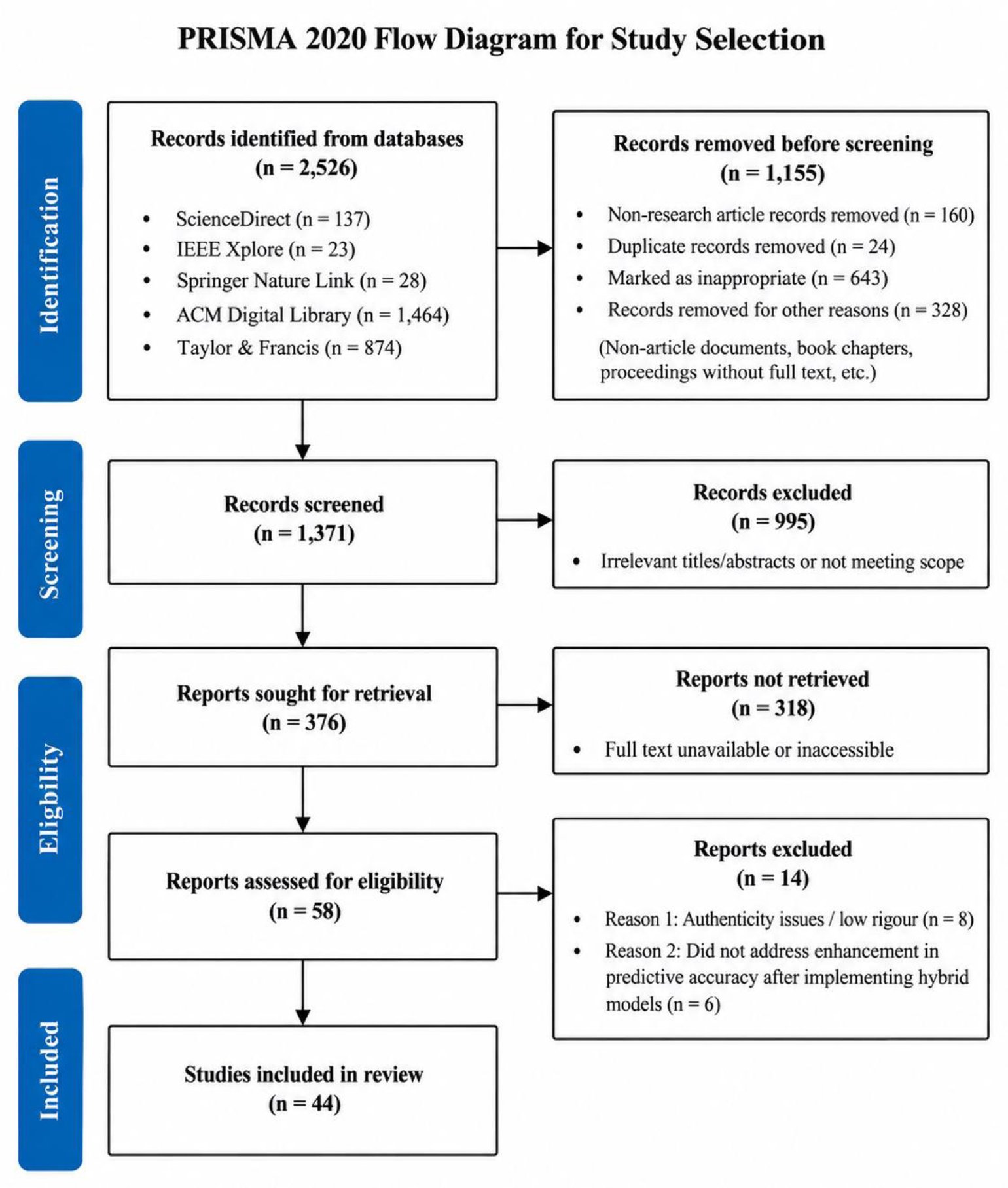
Fig. (1). PRISMA diagram.
Screening and selection were governed by predefined eligibility criteria. Core studies were included when they were peer-reviewed journal or conference articles published in English between 2020 and 2025, addressed multivariate time-series forecasting, operationally integrated at least one statistical component with a deep-learning architecture, and reported quantitative empirical forecasting results. Comparative non-hybrid, univariate, or probabilistic studies were retained only when they served an explicitly labelled contextual or methodological benchmarking role.
Records were excluded when they were non-peer-reviewed or non-English, outside the defined review scope, unrelated to multivariate forecasting, limited to purely statistical or purely deep-learning approaches without operational integration (unless retained as contextual benchmarks), lacked empirical evaluation or standard quantitative metrics, or failed the detailed methodological-quality and relevance checks. Applying these criteria to the 2,526 identified records left 1,371 records for title/abstract screening; 376 advanced to detailed eligibility review, 104 reports were sought for retrieval, 58 full-text reports were assessed, and 44 studies were included in the final synthesis. The stage-specific exclusions are shown in Fig. (1) and reconciled with Table 1. Disagreements were resolved by consensus, full-text exclusions were documented by reason, and quality assessment considered dataset adequacy, baseline adequacy, experimental fairness, and statistical rigour.
Table 1. Database searches and retrieved results.
| Databases | Records Identified | Records Screened After Pre-Screening Removal | Records Retained After Title/Abstract Screening | Records Excluded at Detailed Eligibility Check | Reports Sought for Retrieval | Reports Assessed for Full-Text Eligibility | Selected Studies for Review |
| ScienceDirect (Scopus) | 137 | 121 | 85 | 61 | 24 | 15 | 13 |
| Springer Nature Link | 28 | 20 | 20 | 7 | 13 | 9 | 7 |
| IEEE Xplore | 23 | 16 | 16 | 5 | 11 | 11 | 9 |
| ACM Digital Library | 1,464 | 537 | 130 | 97 | 33 | 11 | 5 |
| Taylor and Francis | 874 | 677 | 125 | 102 | 23 | 12 | 10 |
| Total | 2,526 | 1,371 | 376 | 272 | 104 | 58 | 44 |
2.7. Data Extraction and Quality Assessment
To collect appropriate information on each of the included studies, a formal system of data extraction was used. Data that were extracted included model architecture and hybrid design, dataset characteristics, experimental configuration, baseline comparisons and evaluation metrics. Table A (Appendix A) indicates this information. Table A includes both core hybrid studies and a limited number of contextual benchmark studies. The latter were retained because they provided relevant comparisons concerning baseline performance, cross-variable dependency modelling, forecasting horizons, computational complexity, or deployment feasibility. Their inclusion does not indicate that they satisfy the operational definition of a statistical–deep learning hybrid. In particular, standalone graph-based models and comparative studies that evaluated statistical and deep-learning models separately were not included when deriving the hybrid taxonomy or drawing conclusions about the performance gains of integrated hybrid architectures. This data was used to compare and synthesise the results on the same topic across studies. Also, the predictive performance comparisons reported in this review require careful interpretation because the underlying studies differ substantially in terms of datasets, forecast horizons, evaluation protocols, and baseline model configurations. Although many works report percentage improvements in RMSE, MAE, or MAPE, these values are not directly comparable across studies due to differences in data scale, temporal resolution, domain characteristics, and horizon length, as well as inconsistent choices of statistical and deep learning baselines. For example, short-horizon forecasts on relatively smooth energy or financial series are inherently easier than long-horizon forecasts on noisy, high-dimensional environmental or healthcare datasets, leading to structurally different error distributions even when identical metrics are used. Moreover, several studies tune hybrid models extensively while relying on minimally optimised baselines, further inflating apparent gains. As a result, the reported improvements should be interpreted as directional evidence of relative performance within each experimental context rather than as absolute indicators of superiority across the literature.
A dual-reviewer evaluation methodology was chosen to guarantee the quality of the methodology and reduce subjectivity. Each study was assessed by two independent reviewers in terms of relevance and quality. The inter-rater reliability was evaluated through Cohen’s Kappa coefficient (κ), which yielded a value of 0.6641 shown in Fig. (2) and gave significance to the correlation among the reviewers. Conflicts were resolved by negotiation and agreement.
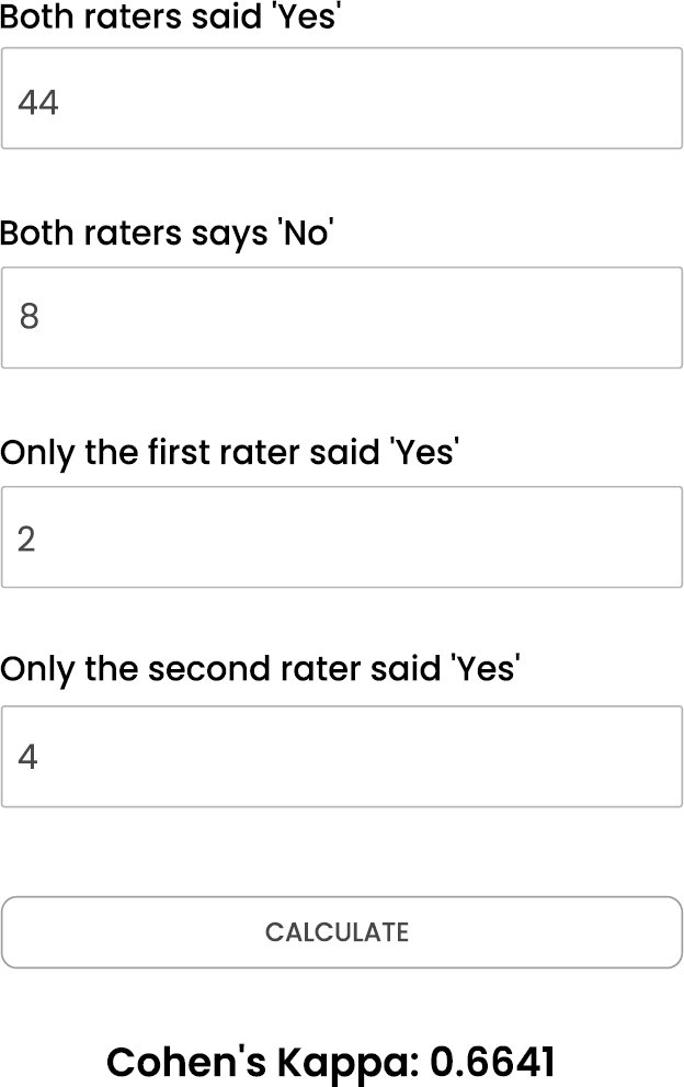
Fig. (2). Cohen’s kappa coefficient calculation [Source: STATOLOGY].
The three major dimensions to which quality appraisal was applied involved reproducibility, experimental rigour, and transparency of the dataset. Studies were evaluated in terms of how well the methodological sections were explained, how satisfactory baseline comparison was, the strength of the evaluation plans, and how report datasets and experimental conditions were presented. This quality evaluation was very strict that the synthesised findings are anchored on sound methodological evidence.
The inter-rater agreement of Cohen’s κ = 0.6641 indicates moderate consistency between reviewers. This reliability measure is operationalised through the above rubric, ensuring that classification into Strong, Medium, and Low evidence categories is not subjective but systematically derived from structured scoring criteria.
Beyond inter-reviewer agreement, a formal methodological rigour assessment was applied to account for heterogeneity in study quality and potential risk of bias. Each included study was evaluated using a structured scoring rubric adapted for forecasting research, covering four dimensions: (1) dataset adequacy and transparency (clear description of variables, frequency, sample size, preprocessing, and public availability), (2) baseline adequacy (use of strong and relevant statistical and deep learning benchmarks rather than weak or outdated comparators), (3) experimental fairness (consistent forecast horizons, rolling or blocked validation strategies, and appropriate train–test splits), and (4) statistical rigor (use of statistical significance testing, ablation studies, or error distribution analysis). Each dimension was scored on a three-level scale (low, medium, high), yielding an overall quality tier classification of strong-, medium-, or low-rigour evidence. This quality-tiering was subsequently used to contextualise reported performance gains, ensuring that conclusions drawn from higher-rigour studies were weighted more heavily than those from exploratory or weakly benchmarked experiments.
3. TAXONOMY OF HYBRID FORECASTING MODELS
Hybrid models that merge the virtues of statistical and Machine Learning (ML) or Deep Learning (DL) algorithms have recently gained popularity in time series forecasting because they can be used to handle complex and non-linear relationships in multivariate data. These models usually combine complementary approaches in enhancing forecasting accuracy, robustness and generalisation capacity. In general, the models based on hybrid approaches can be divided into sequential integration and parallel integration, error-correction and feature-augmentation. The taxonomy of hybrid forecasting models has been critically evaluated in terms of their underlying theoretical mechanisms. A key consideration is the bias-variance trade-off, which explains how hybrid models combine statistical models’ low-variance, high-bias characteristics with deep learning models’ low-bias, high-variance traits to achieve better generalisation. Additionally, inductive bias alignment plays a significant role in determining the success of a hybrid model, with the ability to balance assumptions about the data’s structure (e.g., linearity vs. non-linearity) being critical. Furthermore, the choice between decomposition-based and representation learning-based hybrids is essential for handling different types of time series data. Decomposition methods work well when the data can be naturally separated into components, while representation learning-based hybrids are more flexible, especially for high-dimensional, complex datasets.
Also, sequential integration is the process of using the output of one model as the input of another model, e.g. when a statistical model is used to give initial predictions, which may be optimised using a deep learning model. Parallel integration, on the other hand, is the process that runs several models concurrently and integrates their predictions using processes such as ensemble learning (e.g., averaging, stacking). A sequential hybrid can employ ARIMA (Auto-Regressive Integrated Moving Average) to embrace the linear time series dependence with a network of LSTM (Long Short-Term Memory) to improve the prediction of non-linearities [17, 18]. Conversely, in parallel hybrid models, these two independent models, such as the ARIMA and the LSTM, may be executed simultaneously, and their predictions may be averaged or stacked to generate stronger predictions.
Moreover, there are also error-correction and feature-augmentation hybrid models. The hybrids of error correction are concerned with the fact that the residual errors of one model are used to inform the predictions of a second model, and the residual errors are often learned by a deep learning model that learns the residuals of a statistical model [19–22]. In the meantime, the hybrids of feature augmentation apply the statistical model to the time series to obtain meaningful features and provide them to the deep learning model to make the sophisticated prediction [23, 24]. The two methods serve to increase the prediction power by overcoming the weaknesses of each model, including: statistical models: Cannot represent non-linear dependencies; deep learning models: Cannot classify classical time series behaviours.
3.1. Statistical–Neural Hybrid Architectures
The key to numerous current developments in time series forecasting is hybrid models, which combine neural networks with statistical techniques. ARIMA-LSTM, SARIMA-GRU and VAR-RNN are some examples of such hybrid architectures. These models capitalise on the mathematical capabilities of statistical models and use the predictive ability of neural networks.
3.1.1. ARIMA–LSTM
The ARIMA model is a popular way to model the linear relationships and trend components of the time series data, and the LSTM (a kind of recurrent neural network) is effective to model long-term dependencies and non-linear patterns. This hybrid model takes into account the linear trends and the seasonality of the time series with ARIMA and sends the residual to the LSTM to learn any non-linear trends [25]. The model is effective, especially when the data has non-linear and linear elements.
3.1.2. SARIMA–GRU
Seasonal ARIMA (SARIMA) model is an extension of ARIMA which incorporates seasonal data in the time series. This model can be combined with a GRU (Gated Recurrent Unit), another kind of recurrent neural network, which is useful to model the sequential data with long-term dependencies. SARIMA uses the seasonal and trend factors, whereas GRU can capture the complicated trends in the residuals.
3.1.3. VAR–RNN
Vector Autoregressive (VAR) model is a statistical model that predicts multivariate time series; the variables in the model are supposed to be interdependent. The VAR model could be applied together with an RNN (Recurrent Neural Network) to identify the linear relationships between the variables and optimise them by the RNN to capture non-linear interactions [26]. This hybrid method is especially applicable in predicting multivariate time series when the variables are both linear and non-linear in their relationships.
The mathematical justification of these hybrid models is that the strengths of each of the components are complementary. The statistical model is generally only used to take care of the linear dynamics of the time series, whereas the neural network part is used to capture the complex and non-linear trends. The interplay between these elements is often based on the sequential information flow in which the result of a statistical model is input into the neural network, which then refines the prediction. This architecture uses the strengths of both statistical models and neural networks, as statistical models are more stable and understandable, whereas neural networks are more adaptable and precise.
Hybrid models succeed because the statistical components, such as ARIMA and SARIMA, effectively reduce variance through structured assumptions about the data. These models rely on predefined, simple structures (e.g., linear trends, seasonality), which help minimise overfitting by constraining the possible model fits. In contrast, deep learning components, such as LSTM or GRU, reduce bias by capturing nonlinear dependencies and complex patterns in the data that traditional statistical models often miss. This synergy between the two paradigms directly complements the classical bias-variance trade-off in forecasting. By combining the strengths of both, hybrid models balance the tendency of statistical models to underfit (high bias) with the ability of deep learning models to overfit (high variance), thus achieving improved generalization and predictive accuracy, especially in complex multivariate time series forecasting tasks.
3.2. Taxonomy of Statistical–Deep Learning Hybrid Forecasting Models
Statistical–deep learning hybrid forecasting models combine the interpretability and structured modelling capability of statistical approaches with the nonlinear pattern-learning ability of deep learning architectures. However, existing studies use the term “hybrid” to represent different integration strategies, including residual learning, feature extraction, ensemble combination, and optimisation-based improvement. To provide a consistent classification framework, this review categorises hybrid forecasting approaches into four major types: residual/error-correction hybrids, feature-level hybrids, ensemble hybrids, and optimisation hybrids.
3.2.1. Residual/Error-Correction Hybrid
Residual hybrid models use a statistical forecasting model to generate an initial prediction, while a deep learning model learns the remaining forecasting errors or residual patterns. This approach enables statistical models to capture linear trends, seasonality, and historical dependencies, whereas deep learning models identify complex nonlinear relationships that remain unexplained. Common examples include ARIMA–LSTM, SARIMA–GRU, and VAR–RNN architectures.
3.2.2. Feature-Level Hybrid
Feature-level hybrid models integrate statistical information as additional input features for deep learning models. Instead of directly predicting residual errors, statistical methods extract meaningful characteristics such as trends, seasonal patterns, lag relationships, or decomposed components, which are subsequently used by deep learning architectures to improve forecasting capability. Examples include VAR-derived features combined with LSTM models and statistical decomposition techniques integrated with CNN architectures.
3.2.3. Ensemble Hybrid
Ensemble hybrid models combine predictions from multiple forecasting approaches to improve robustness and reduce individual model limitations. These approaches integrate statistical and deep learning forecasts through techniques such as averaging, weighted aggregation, or stacking methods. By combining different predictive perspectives, ensemble hybrids improve generalisation, particularly when datasets contain multiple temporal patterns or uncertain behaviour.
3.2.4. Optimisation Hybrid
Optimisation hybrid models incorporate optimisation algorithms to enhance model configuration, parameter selection, or architecture performance. These approaches improve hybrid forecasting by automatically identifying suitable hyperparameters, model structures, or feature combinations. Common optimisation methods include Bayesian optimisation, genetic algorithms, and particle swarm optimisation, which are applied to improve forecasting accuracy while managing model complexity.
The classification framework enables systematic comparison of hybrid forecasting approaches by distinguishing the mechanism through which statistical and deep learning components are integrated (Table 2).
Table 2. Classification of statistical–deep learning hybrid forecasting models.
| Study | Hybrid Category | Statistical Component | Deep Learning Component | Application |
| Mohideen et al., [10] | Type I: Residual/Error-Correction Hybrid | ARIMA | LSTM | Weather forecasting |
| Guillamet et al., [11] | Type II: Feature-Level Hybrid | Statistical lag features | LSTM | Healthcare demand forecasting |
| Guermoui et al., [25] | Type IV: Optimisation Hybrid | VMD/statistical decomposition | CNN | Solar forecasting |
| Padilha et al., [30] | Type IV: Optimisation Hybrid | SARIMA | LSTM + optimisation algorithm | Wind forecasting |
| Tejoyadav et al., [36] | Type I: Residual/Error-Correction Hybrid | VAR | LSTM | Water quality forecasting |
| Lian & Tian [41] | Type III: Ensemble Hybrid | Statistical forecasting models | Deep learning models | Air quality forecasting |
3.3. Residual and Error-Driven Hybrid Models
Residual learning is one of the most widespread approaches to combining statistical models with deep learning: the statistical model is used to make the baseline prediction, and a deep learning model is used to make the prediction of the difference between the actual values and the baseline. This combination model structure is effective in solving the bias-variance trade-off in time series forecasting.
Under this context, statistical models (ARIMA or SARIMA) give a very good but not always accurate prediction using linear trends and past data. Then, the deep learning model (LSTM, GRU or CNN) is aimed at learning the residuals, i.e., the differences between the forecast and the actual observations, and optimising the forecast. The advantages of this architecture include the storage and processing of structured, linear data with the use of the statistical model and non-linear and difficult-to-learn relationships with the use of a deep learning model. The major benefit of residual learning is that it minimises the bias without causing a huge variance that would pose inaccurate predictions in the presence of noise or outliers. According to the research by [27] and [28], the baseline of ARIMA or SARIMA is followed by the error correction stage using LSTM or GRU, and it results in increased accuracy of the forecasting results, especially when the data is subjected to non-linear processes or irregularities.
The review developed an explicit decision-oriented framework by linking dataset characteristics with appropriate hybrid forecasting strategies. The framework mapped key data properties, including dataset size, dimensionality, noise levels, and forecasting horizon, to suitable model selection approaches. A structured decision process was established to support evidence-based hybrid model selection rather than relying solely on descriptive comparisons. This framework enhanced the practical relevance of the review by providing clearer guidance on the conditions under which different hybrid forecasting architectures were most appropriate.
3.4. Feature-Level and Ensemble Hybridisation
The other popular method of hybrid forecasting models is feature-level hybridisation and ensemble learning. In feature-level hybridisation, the statistical models are utilised to create features (trends, seasonality, correlations, etc.) out of the time series data and input them into deep learning models in order to make additional predictions. This is a good strategy as it enables the deep learning model to concentrate on learning intricate patterns, whereas the statistical one makes sure that the key characteristics of the data are learned at the initial stage of the procedure.
For instance, a SARIMA-LSTM hybrid can be used by initially running SARIMA to obtain seasonality and trend characteristics that are subsequently fed into LSTM to generate the residual to refine the forecasts. Such hybridisation is useful to make sure the linear and non-linear components of the time series are captured, which leads to more accurate predictions. As shown by [29] and [30], statistical characteristics, e.g., autocorrelations or seasonality components, can improve the LSTM model in terms of the capacity to learn more of the deep non-linear relationships.
Ensemble techniques such as stacking, bagging and boosting also enhance the accuracy of the forecasts by summing the results of the other models, be it statistical or based on machine learning, into a single aggregated forecast [31–36]. The process of ensemble averaging averages the predictions made by a number of models and serves to smooth out the biases of single models. Stacking, in its turn, is based on a meta-model that combines predictions of base models to achieve an improved performance [37–39].
Kumar and Singh [40] demonstrate the usefulness of ensemble hybridisation, in which several statistical models, as well as deep learning techniques, are jointly used. The ensemble model has the capability to utilise the complementary advantages of the individual models and produce stronger and more credible forecasts, especially when the dataset has different patterns and trends. In studies such as [41, 18], statistical and deep learning methods are explicitly combined through multivariate combination and comparative forecasting frameworks. Attention, graph learning, or optimisation mechanisms are included only when embedded within hybrid structures, as seen in [42] and [43]. Pure models such as standalone Transformer-based approaches in [44, 45, 46], they are excluded unless integrated with statistical components, ensuring strict methodological boundaries and preventing scope drift across heterogeneous forecasting frameworks.
3.5. When Hybrid Models May Not Be Appropriate
Although hybrid statistical–deep learning models generally demonstrate improved forecasting performance, their application is not universally suitable. In several contexts, hybridisation may introduce unnecessary complexity without proportional performance gains. Firstly, in scenarios involving small datasets, deep learning components are prone to overfitting due to insufficient training samples, resulting in unstable or non-generalizable predictions. In such cases, simpler statistical models often perform more reliably.
Secondly, for highly stationary processes, traditional statistical models such as ARIMA or SARIMA may already capture the underlying structure effectively, making hybridisation redundant and computationally inefficient. Thirdly, in low-latency or real-time forecasting environments, the computational overhead introduced by hybrid architectures, particularly those involving deep learning or ensemble components, may limit practical deployment feasibility. Finally, in resource-constrained settings, including edge devices or systems with limited memory and processing power, hybrid models may be impractical due to high training and inference costs. Therefore, hybrid forecasting models should be selected conditionally, based on dataset characteristics and operational constraints, rather than assumed to be universally superior.
Each thematic subsection concludes with a concise synthesis summarising the dominant empirical pattern observed across studies, the overall strength of supporting evidence, and any inconsistencies or disagreements within the literature. It further highlights the implications for forecasting practice, particularly in terms of model selection, performance reliability, and contextual suitability. This ensures that descriptive summaries are advanced into analytical interpretation, improving coherence, critical depth, and methodological contribution across thematic discussions.
4. COMPARATIVE ANALYSIS OF PREDICTIVE PERFORMANCE
4.1. Evaluation Metrics Used
In time series forecasting, an evaluation metric is an essential concept that determines how a particular model can perform and its accuracy. Root Mean Squared Error (RMSE), Mean Absolute Error (MAE) and Mean Absolute Percentage Error (MAPE) are commonly employed measures in the literature. These measures have become popular due to the fact that they give information on the scale of error in prediction and can be easily interpreted, especially where forecasting tasks are considered in which the minimisation of prediction error is the most important aspect.
4.1.1. RMSE
This is a measure that is computed as the square root of the mean of the squared error between actual and predicted values. RMSE is very sensitive to big errors, and it is applicable in measuring models where big deviations of the true values are an issue of great concern. The RMSE value is also going to be generally much better in hybrid models, which can address non-linear dependencies that statistical models might not address [47].
4.1.2. MAE
The MAE is the mean of the absolute deviations between the actual and the predicted values. In contrast to RMSE, MAE provides a linear grade and does not prioritize any error, which can be advantageous in the situation when outliers are not so essential. Research, including that of [48, 49] has shown that hybrid models tend to have lower MAE values because of a combination of the capacity to model both linear and non-linear aspects of the data.
4.1.3. MAPE
This measure of error is expressed as a percentage, which is easy to interpret across the various datasets. However, MAPE is also deceptive when the actual values are near zero because even minor variations can cause huge percentage errors.
In the case of multivariate time series, these measures are generalised to cover many variables. Multivariate RMSE (MRMSE) and Multivariate MAE (MMAE) are commonly computed by summing up the errors of individual time series variables. The metrics can be used to measure the models in an environment where several interdependent time series need to be forecasted at once [50]. Also, the performance of the forecasting models is usually different when the forecast horizon is considered, so horizon-specific accuracy is also essential.
While RMSE, MAE, and MAPE are commonly used metrics in evaluating hybrid forecasting models, they have known drawbacks that can distort the interpretation of model performance (Fig. 3). RMSE is sensitive to outliers and can exaggerate the impact of large errors, particularly in datasets with extreme values, while MAE is scale-dependent and may not be suitable for comparing models across different datasets with varying scales. MAPE, although widely used, suffers from instability when the true values are close to zero, making it unsuitable for datasets with rare or small values. Despite these limitations, these metrics remain dominant due to their simplicity and ease of use, particularly when comparing hybrid models to traditional statistical models. However, focusing solely on accuracy measures like RMSE, MAE, and MAPE overlooks important factors like distributional metrics and model calibration, which are critical for evaluating forecast uncertainty and the overall superiority of hybrid models. Future evaluations should include probabilistic scores, such as Brier score or CRPS, and interval-based metrics to provide a more comprehensive view of a model’s forecasting capability. While accuracy remains important, hybrid models’ effectiveness should also be assessed by their ability to handle uncertainty and produce reliable, actionable predictions across dynamic datasets.
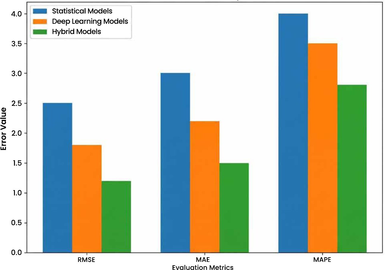
Fig. (3). Performance comparison based on evaluation metrics.
4.2. Static vs Streaming Data Environments
The review currently merges studies using static datasets with those operating in streaming or dynamic environments, despite fundamental differences in data generation and model adaptability requirements. Static datasets typically assume fixed distributions and are suitable for batch-trained hybrid models, while streaming environments require continual learning, adaptability, and low-latency updates. Mixing both contexts weakens interpretability of comparative findings. A classification scheme should therefore be introduced to separate static and streaming-based applications within the synthesis framework. This distinction will clarify model suitability, highlight adaptation requirements, and improve the validity of conclusions regarding hybrid forecasting performance across real-world operational conditions.
4.3. Benchmarking Against Standalone Models
Standalone models are frequently used to benchmark the performance of hybrid models (e.g., pure statistical models i.e. ARIMA, VAR and pure deep learning models i.e. LSTM, GRU). Hybrid models, these are models that integrate the advantages of the statistical and deep learning approaches; such models have been shown to perform very well on forecasting activities. Another instance of benchmarking is that the deep learning models usually succeed in the management of non-linearity and intricate interactions compared to the traditional statistical models. Nevertheless, hybrid models take the merits of both methods and result in more accuracy and strength. As an illustration, [17] note that the RMSE has reduced by a quarter when a hybrid model of deep learning and statistical methods is used over the same model applied to each method separately. Market trends are volatile, and the hybrid models in financial forecasting have been particularly useful in ensuring that predicted data is smooth without making it volatile due to the use of both classic trend-following approaches and complex pattern recognition.
Hybrid models are far more successful than pure statistical and pure deep learning models in terms of the accuracy improvements that they have, particularly in tasks with long-term predictive requirements, as illustrated in Fig. 4. Hybrid models are more likely to be more accurate because they combine interpretability and simplicity of statistical models and the flexibility and ability of deep learning models to parameterise complex non-linear associations.
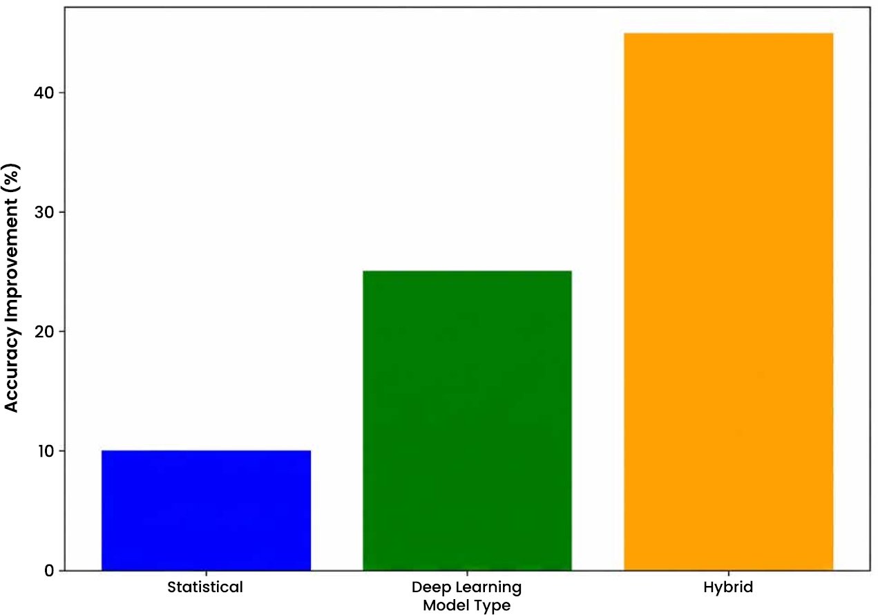
Fig. (4). Benchmarking hybrid models against standalone models.
4.4. Computational Trade-offs (Latency, Cost, Memory)
To evaluate forecasting accuracy, practical deployment of hybrid statistical–deep learning models also depends on computational requirements. Hybrid models generally achieve improved predictive performance by combining statistical stability with deep learning flexibility; however, this improvement often involves higher training complexity, memory consumption, and computational costs. Therefore, model selection should consider the balance between forecasting accuracy and operational feasibility (Table 3).
Table 3. Computational and deployment trade-offs of forecasting models.
| Factor | Statistical Models | Deep Learning Models | Hybrid Models |
| Training Cost | Low | High | Medium–High |
| Computational Requirement | Low | High | High |
| Interpretability | High | Low | Moderate |
| Forecast Accuracy | Moderate | High | High for complex datasets |
| Deployment Complexity | Low | Medium | High |
This analysis highlights that hybrid models are most suitable for large, complex, and nonlinear forecasting problems, whereas simpler approaches may remain preferable for applications requiring low latency and limited computational resources.
4.5. Forecast Horizon–Based Performance Differences
The reviewed studies demonstrated that forecasting performance varied considerably across short- term, medium- term, and long-term horizons. The analysis indicated that forecasting horizon influenced error propagation, model stability, and the ability of different architectures to capture temporal dependencies. Short-term forecasting studies generally achieved strong performance using statistical and lightweight hybrid approaches because of lower uncertainty and limited dependency requirements. Medium-term forecasting applications benefited from hybrid models that effectively combined statistical trend extraction with deep learning-based residual learning. In contrast, long-term forecasting tasks demonstrated greater reliance on advanced deep learning and decomposition-based hybrid architectures due to their ability to capture complex and long-range temporal relationships (Table 4).
Table 4. Forecast horizon-based performance comparison of hybrid models.
| Forecast Horizon | Typical Applications | Effective Models | Key Finding |
| Short-term | Traffic, weather, finance | CNN–LSTM, GRU hybrids | Effective in capturing short-term nonlinear patterns and rapid changes |
| Medium-term | Healthcare demand, energy forecasting | ARIMA–LSTM, VAR–LSTM | Improved trend and residual pattern modelling |
| Long-term | Electricity, climate, large-scale forecasting | Transformer-based hybrids | Better learning of long-range temporal dependencies |
A comparative synthesis was conducted by examining forecasting horizon, dataset quality, baseline adequacy, experimental fairness, and statistical rigor across the selected studies. The assessment indicated variation in methodological strength among reviewed studies, with some studies providing stronger evidence through transparent datasets, comprehensive baseline comparisons, robust validation procedures, and advanced statistical evaluation (Table 5).
Table 5. Evidence quality assessment of reviewed studies.
| Study | Dataset Quality (1–3) | Baseline Adequacy (1–3) | Experimental Fairness (1–3) | Statistical Rigor (1–3) | Total Score (4–12) | Evidence Level |
| [19] | 2 | 2 | 2 | 2 | 8 | Medium |
| [20] | 3 | 3 | 3 | 2 | 11 | Strong |
| [21] | 2 | 3 | 2 | 2 | 9 | Medium |
| [22] | 2 | 3 | 2 | 2 | 9 | Medium |
| [26] | 2 | 2 | 2 | 1 | 7 | Medium |
| [33] | 2 | 3 | 2 | 2 | 9 | Medium |
| [34] | 3 | 2 | 3 | 2 | 10 | Strong |
| [35] | 2 | 2 | 2 | 1 | 7 | Medium |
| [46] | 3 | 3 | 3 | 3 | 12 | Strong |
4.6. Dataset Characteristics and their Impact
The suitability of the datasets used has a significant effect on the performance of the hybrid models. Some of the common attributes that influence the predictive power of hybrid models are stationarity, dimensionality and noise.
4.6.1. Stationarity
Stationarity is a set of statistical characteristics of a time series being unchanged with time, including the mean and the variance. Hybrid models, especially those which incorporates statistical elements such as ARIMA are more suitable with stationary time series whereby the underlying patterns do not shift radically with time. Nevertheless, when non-stationary data are considered, deep learning models, in particular LSTM, can be especially useful, as a lack of stationarity is not assumed, and they are able to extract patterns in data that change with time.
4.6.2. Dimensionality
Multivariate time series can include many variables, which may have a major impact on the model. The hybrid models, including VAR-LSTM and SARIMA-GRU, are especially useful when dealing with high-dimensional data as they consist of the benefits of statistical models in addressing inter-variable correlation with the potential of deep learning models to work with large volumes of input data. As it was shown by [50], hybrid models trained on high-dimensional data sets (i.e. energy consumption data with a high number of influencing factors) always performed better than univariate or even multivariate models.
4.6.3. Noise
Noise in time series data is the random variation which is not based on the underlying patterns. The hybrid models are also most useful when dealing with noisy data since the deep learning techniques can learn a large set of data and determine trends that statistical approaches may fail to detect.
The analysis of hybrid models’ performance across data regimes is discussed in Table 6 below.
Table 6. Hybrid model performance across data regimes.
| Hybrid Model Type | Data Regime | Forecast Horizon | Performance Stability | Key Findings |
| LSTM–ARIMA | Noisy, low-dimensional | Long-term (> 1 year) | Low when noise dominates | Hybridization adds complexity without performance gains in high-noise environments (7) |
| ARIMA–LSTM | Stationary, low-dimensional | Short-term (1–12 months) | High, but fluctuates with noise | Outperforms ARIMA, but LSTM component may struggle with very short-term forecasts (17) |
| SARIMA–GRU | Non-stationary, high-dimensional | Long-term (1–5 years) | Stable, excellent in handling seasonality | Significant improvements over standalone SARIMA, especially for non-linear trends (22) |
| SARIMA–CNN | Stationary, low-dimensional | Short-term | High stability | Effective in modeling short-term forecasts, but CNN component struggles with long-term dependencies (25) |
| VAR–RNN | Multivariate, high-dimensional | Medium-term (6–24 months) | Stable for financial and energy forecasting | Robust for capturing cross-variable dependencies, but computationally expensive (46) |
4.7. Failure-Mode Analysis of Hybrid Models
In this review, hybrid models are often heralded for their ability to improve forecasting accuracy. However, in certain contexts, hybrid models fail to outperform simpler statistical models or deep learning methods. Failure-mode analysis reveals several situations where hybridization may not be beneficial.
4.7.1. Overfitting
Hybrid models that include deep learning components, such as LSTM or GRU, may overfit when training data is limited, leading to poor generalization. This issue is particularly evident in domains like financial forecasting, where volatility and noise can cause LSTM-based hybrids to memorize noise rather than capture meaningful patterns.
4.7.2. Increased Computational Complexity
In cases where the dataset is low-dimensional, hybrid models involving complex deep learning layers (e.g., LSTM or CNN) may increase computational costs without offering a corresponding improvement in accuracy. For example, in short-term forecasting applications where ARIMA alone suffices, hybridization may lead to unnecessary complexity and longer training times.
4.7.3. Poor Performance in Noisy Data
Hybrid models, especially those that integrate statistical methods with deep learning, may fail to improve accuracy in highly noisy environments. The additional deep learning layer may struggle to filter out noise effectively, leading to minimal performance improvements compared to pure statistical models.
4.7.4. Non-Improvement in Short-Horizon Forecasting
When the forecast horizon is short-term, deep learning models often struggle to provide significant improvements over traditional statistical models, which can capture immediate temporal dependencies more effectively. For example, ARIMA models frequently outperform hybrid models for short-term forecasts in stable, low-dimensional datasets.
4.8. Computational and Practical Considerations
Although hybrid models have an important advance in terms of accuracy, there are also some computation and practical issues that have to be resolved. These are training cost, model interpretability and feasibility of deployment.
4.8.1. Training Cost
Hybrid models, particularly models with deep learning elements may be computationally costly to train. Deep learning model training, be it LSTM or GRU, takes a large number of computational resources and time, particularly in the case of large datasets. Such models as LSTM-ARIMA hybrids may need hours or even days of training time based on the size of the dataset. This is unlike the traditional statistical models which are usually very fast and less computationally intensive. Nevertheless, hybrid models tend to have more advantages in terms of accuracy than the increased training costs depending on the complexity of the task of forecasting, and in situations where the quality of prediction is the most important criteria.
4.8.2. Interpretability
Deep learning models are powerful models with a high probability of lacking interpretability, and it is challenging to know how the model is arriving at the predictions. This is a crucial problem in areas like finance and healthcare where decision-making processes of the predictions should be known to the stakeholders. Thus, it is possible to find a compromise between the precision of deep learning and the explainability of statistical tools in the hybrid models.
4.8.3. Deployment Feasibility
Hybrid models may be difficult to deploy in real-life applications because the models are more complex and require more computation. Nevertheless, hybrid models can be implemented in real-time decision-support systems. The added complexity of the hybrid models is warranted in such applications by the enhancement in the forecasting accuracy. Also, hybrid models enjoy the support of developments in cloud computing and distributed processing that can be used to alleviate the difficulties of deploying the models through scalable and efficient execution of the model.
Table 7 below summarises the properties of datasets and computation of some of the selected hybrid models surveyed.
Table 7. Dataset characteristics and their impact on hybrid models.
| Ref. | Study [Authors (Year)] | Dataset Characteristics | Stationarity | Dimensionality | Noise | Computational Cost | Interpretability | Deployment Feasibility |
| [11] | (Hernández Guillamet et al., 2025) | Healthcare demand | Stationary | Medium | Moderate | High | High | Low |
| [20] | (Liu et al., 2025) | Financial, energy | Non-stationary | High | Low | High | Moderate | High |
| [21] | (Zheng & Lucey, 2025) | Stock market | Non-stationary | Medium | High | High | Low | Moderate |
| [22] | (Lei et al., 2025) | Traffic, energy | Non-stationary | High | Low | High | Moderate | High |
| [23] | (Sriramulu et al., 2025) | Stock market | Non-stationary | High | High | High | Low | Moderate |
5. DISCUSSION
5.1. Key Insights from the Review
The synthesis comprised core statistical–deep learning hybrid studies together with a limited set of explicitly identified contextual benchmark studies. Conclusions concerning hybrid architecture, integration mechanisms, and forecasting gains were based primarily on the core hybrid evidence, while comparative and graph-based benchmark studies were used only to contextualise baseline performance, cross-variable modelling capability, computational trade-offs, and conditions under which hybridisation may not be necessary.
The high performance of hybrid models is attributed to the fact that they are able to identify both the linear and non-linear dependencies. ARIMA and VAR are good statistical models for modelling linear trends, seasonality, and stationarity in time series data, as was shown in research by [6, 20]. Deep learning models, including LSTM or GRU, on the other hand, are better at capturing non-linear dependence and long-term dependence that are often missing in statistical models. All these complementary strengths are taken advantage of by these hybrid models, and hence they are very versatile and can produce more accurate predictions. Indicatively, [24] established that hybrid systems such as ARIMA to capture linear and LSTM to refine non-linear forecasts of financial time series yielded better financial time series forecasting accuracy than non-hybrid ARIMA and LSTM regression systems.
ARIMA-LSTM and SARIMA-GRU stand out as some of the most prevalent architectures to work with since it gives a solid framework for addressing both short-term dynamics and intricate non-linear interactions. As an example, Liu et al., [20] observe that this hybrid combination is effective in energy forecasting, in which ARIMA models deal with the linear tendency, and LSTM networks address the sophisticated temporal relationships that arise in the residues. Lei et al., [22] also focus on the prevalence of graph-based hybrid models such as METRO (GNN), which use temporal-spatial graphs to predict multivariate time series in the domains of traffic and energy. Such architectures are also being strongly favoured due to the fact that they are more suited to support the interdependency between two or more time series variables, which is a common feature of real-world applications.
5.2. Statistical Interpretability vs Deep Learning Flexibility
One of the main themes that can be identified in the review is a trade-off between statistical interpretability and flexibility of deep learning. It is a generally accepted opinion that statistical models are more transparent and interpretable. To illustrate, ARIMA models are founded on mathematical concepts that have known principles, and their coefficients can be interpreted in most cases to explain how past values affect future predictions. Such an interpretable level is essential in such research areas as finance and healthcare, where interested parties require comprehending the logic of forecasts. According to [17], this transparency is a considerable benefit of statistical models, particularly when the regulatory or decision-making authorities demand an unambiguous answer to the way to get a particular forecast. Deep learning models, including LSTM and GRU, on the contrary, allow more flexibility in the modelling of complex patterns, particularly non-stationary, high-dimensional data [24]. This flexibility, however, comes with the trade-off of interpretability. The deep learning models are usually referred to as black-box models since it is a hard task to follow how certain inputs can produce certain outputs. This non-transparency is a major challenge to the explainability of what the model predicts, particularly in areas such as healthcare, where interpretation of model decisions is a key element in terms of trust and safety.
The hybrid strategy tries to find a compromise between these conflicting requirements. Hybrid models provide an avenue to higher accuracy and, at the same time, exhibit some degree of interpretability by providing the statistical rigour of the ARIMA or SARIMA models with the flexibility of the deep learning models. According to Mishra et al., [7], deep learning models alone might be more accurate in their predictions compared to the conventional approach, but the hybrid variant provides a more intuitive approach with no performance loss.
Nevertheless, explainability is still an issue even in hybrid models. As emphasised by Zhao et al., [46] the hybrid model can lead to superior results; however, it does not necessarily make the deep learning aspect more interpretable. The interpretability offered by the statistical model of a hybrid approach is accompanied by the fact that the deep learning aspect is always complicated, and there is still a need to develop explainable AI (XAI) methods to ensure that such models can be trusted and implemented in sensitive matters.
5.3. Performance Mechanisms and Variation Across Hybrid Models
The reviewed studies indicated that hybrid statistical–deep learning models improved forecasting performance by combining complementary modelling capabilities. Statistical components reduced forecasting bias by capturing linear trends, seasonality, and historical dependencies, while deep learning components improved nonlinear pattern recognition and residual error correction. These advantages were particularly evident in high-dimensional datasets, noisy environments, and forecasting problems involving complex nonlinear relationships.
However, differences in reported performance occurred due to variations in dataset characteristics, baseline model selection, forecasting horizons, and validation strategies. Models demonstrated stronger improvements when evaluated on large, complex datasets with appropriate benchmark comparisons, whereas simpler datasets or weaker validation approaches produced less consistent results. Therefore, hybrid model effectiveness depended not only on architecture selection but also on the characteristics and requirements of the forecasting problem.
5.4. Methodological Limitations in Existing Studies
Although the outcomes of the studies reviewed are promising, the methodological limitations which complicate the generalizability and the strength of findings are quite a few. The use of small datasets is one of the greatest problems. Numerous studies, especially those in small domains such as healthcare forecasting or environmental prediction, use small datasets, which might not fully address the variability of the real-world phenomenon that it seeks to model. A point raised by Khosravi et al., [6] was the possibility of overfitting in hybrid models due to inadequate data, because a model may work well on the training data but fail to effectively generalise to novel and unexplored data. This weakness underscores the significance of larger and more heterogeneous datasets to test hybrid models, particularly when using applications such as energy forecasting or financial prediction, where data is more likely to be richer and more fluid.
The other major concern is the fact that benchmarking in studies is not consistent. Although most of the studies use RMSE and MAE as measures of evaluation, there is not much consistency in the selection of the baseline models with the aim of comparison. He et al., [24] highlighted that the comparison of hybrid models to pure statistical or pure deep learning models is not necessarily justified and standardised when it comes to the choice of baselines. This lack of consistency complicates arriving at conclusive findings on the effectiveness of the hybrid models in various fields.
In addition, many of the hybrid model papers do not involve ablation studies, and thus it is impossible to determine the contribution of each component of the hybrid model to overall performance. Mishra et al., [7] observe that hybrid models are likely to perform better than standalone models, although the role of the deep learning component compared to the statistical component cannot be established without ablation studies. The execution of such studies would assist in drawing clarity on the contribution of various elements of a hybrid model to accuracy gains and assist practitioners to choose the appropriate combination of elements in their particular forecasting assignment.
5.5. Implications for Machine Learning and Statistics
Hybrid modelling is a transmission of traditional models to state-of-the-art machine learning techniques, providing a new approach to the problems of making predictions based on multivariate time series. Because statistical methods like ARIMA or VAR can be used to combine with deep learning models, like LSTM or CNN, such hybrid systems are useful in modelling both linear and non-linear relationships in the data. This integration greatly increases the prediction power of time series forecasting models and provides a wide range of application potential in different fields, such as finance, energy, health and environmental care [50].
Hybrid models can be important to explainable AI (XAI), exposing deep learning approaches to a greater level of interpretability. Although deep learning models are frequently criticised because of being black-box models, hybrid models that integrate statistical methods provide an avenue through which predictions can be explained. ARIMA models would, as an example, be able to give an understanding of the trend and seasonality of the data, which can be complemented by the deep learning model, which can represent intricate non-linear trends. This may be used to address the discrepancy between accuracy and explainability, which is a critical factor in such a domain as healthcare, where it is vital to understand the transparency of AI decisions used. In addition, hybrid models stand at the right spot to deal with numerous real-life issues in predictive applications.
5.6. Open Challenges and Future Research Directions
Hybrid forecasting techniques that combine both statistical and deep learning techniques have proven highly effective in enhancing predictive accuracy on Multivariate Time Series (MTS). Nevertheless, with the field’s development, several unresolved issues are still open, and they may influence the trend of future research. The scalability of hybrid models to high-dimensional multivariate time series is one of the leading challenges. The so-called curse of dimensionality is the exponential increase in computational cost and data demands as the size of the feature set or time series variables is enlarged. Financial and other energy prediction Data of high dimensionality can result in models that are computationally expensive and overfitted. High-dimensional data applications such as stock market prediction or environmental observing. Various methods that could be investigated in the future to address these difficulties include Principal Component Analysis (PCA), autoencoders, or sparse learning to enable hybrid models to be more effective in large-scale, high-dimensional applications.
The explainability and model transparency of hybrid models, especially those that include deep learning elements such as the LSTM or GRU, is also another important challenge. Although these models may provide high predictive power, they are usually black-box models, in which the reasons that are used to make the predictions are hard to decipher. Such interpretability has been a major challenge in other areas like healthcare, where knowing how AI has made decisions is fundamental to user trust and clinical implementation. Transformers with attention has become a major trend in time series forecasting, especially since 2022. Transformers were initially created as a Natural Language Processing (NLP) application, having been shown to be capable of modelling long-range dependencies and long-range complex temporal patterns in sequential data. Future studies are supposed to investigate the ways that these Transformer-based architectures can be extended with custom statistical models in order to improve their capabilities of handling large and complex-sized datasets and thus progress the state of the art in long-term forecasting.
Finally, the attempt to create automated hybrid model selection by means of AutoML (Automated Machine Learning) and Bayesian optimisation methods can be considered as one of the most promising research directions in the future. AutoML systems could potentially automate the procedure of choosing optimal model architectures and hyperparameters for a particular task, drastically decreasing the amount of time and experience one needs to build a model. Further evolution of these methodologies will make the hybrid forecasting models more flexible and accessible and be able to apply to larger and more complex datasets, making the predictions of these models more transparent, interpretable, and optimised. Finally, the concerns of scalability, explainability, transformer integration, and automated model selection will provide new opportunities for hybrid models to achieve substantial improvements in time series forecasting in the broad scope of domains.
5.7. Future Research Directions
Future research should address several methodological gaps identified in the reviewed literature. First, greater attention is required toward uncertainty-aware hybrid forecasting, as many existing studies focus only on point prediction without providing prediction intervals or confidence estimation. Second, external validation remains limited, with many models evaluated only on specific datasets or single application domains, restricting generalisability. Third, improved reproducibility is needed through transparent reporting of datasets, model parameters, and publicly available implementations. Fourth, future studies should incorporate deployment benchmarking by evaluating computational cost, inference speed, memory requirements, and scalability. Finally, the development of adaptive hybrid models for streaming data environments is needed to address concept drift, continuous learning requirements, and real-time forecasting challenges.
CONCLUSION
This is a systematic literature review that summarises the current developments in hybrid statistical-deep learning models of multivariate time series forecasting. The main results indicate the great benefits of hybrid models in enhancing the accuracy of forecasting in several fields, such as finance, energy, health, and environmental monitoring. Recent hybrid models, that is, models based on a mixture of statistical algorithms such as ARIMA, SARIMA and VAR and deep learning algorithms such as LSTM, GRU, and CNN, leverage the advantages of both paradigms in an attempt to resolve the complexities of multivariate time series data. All of these models provide a good tradeoff between being linear and non-linear, providing an opportunity to capture short-term dependency and long-range temporal relationships in a much better way than single models.
Using the reviews of 44 studies, it is easy to find that hybrid models are always better than either pure statistical models or pure deep learning models. In particular, it was common to find that ARIMA-LSTM and SARIMA-GRU hybrids performed well in terms of modelling linear trends and seasonality, whereas deep learning elements performed well in terms of modelling non-linear dependencies and long-term effects. Not only does the addition of predictive power from multivariate time series models contribute, but the contribution of this review also has some value to the increasingly growing research in the area of statistics-driven Machine Learning (ML). Using classical statistical models and contemporary deep learning models, this work draws attention to the possibility of hybrid models serving as an intermediary between the two spheres. Overall, hybrid forecasting models can be considered as a potent and adaptable means of multivariate time series forecasting. They provide major advancements in predictive accuracy, strength, and extrapolation in different fields. Nevertheless, issues still exist, especially in scalability, interpretability and efficiency of the models, which have to be tackled in future studies. The area of hybrid models can only improve as deep learning continues to develop and as transformer-based architectures and automated model selection tools such as AutoML are integrated, which should further improve the performance and accessibility of hybrid models. In this review, the future of hybrid models has been highlighted as promising and can potentially bring a revolution in the field of forecasting in multifaceted, high-dimensional areas.
LIST OF ABBREVIATIONS
ARIMA | = | Autoregressive Integrated Moving Average |
AutoML | = | Automated Machine Learning |
CNNs | = | Convolutional Neural Networks |
DL | = | Deep Learning |
DNNs | = | Deep Neural Networks |
GRUs | = | Gated Recurrent Units |
LSTMs | = | Long Short-Term Memory Networks |
MAE | = | Mean Absolute Error |
MAPE | = | Mean Absolute Percentage Error |
ML | = | Machine Learning |
MMAE | = | Multivariate MAE |
MRMSE | = | Multivariate RMSE |
MTS | = | Multivariate Time Series |
NLP | = | Natural Language Processing |
PCA | = | Principal Component Analysis |
PRISMA | = | Preferred Reporting Items for Systematic Reviews and Meta-Analyses |
RMSE | = | Root Mean Squared Error |
SARIMA | = | Seasonal ARIMA |
SLR | = | Systematic Literature Review |
VAR | = | Vector Auto-Regression |
AUTHOR’S CONTRIBUTION
O.R. contributed to the conceptualization and study design, development of the methodology, data collection, analysis and interpretation of the results, drafting of the manuscript, and critical revision of the final manuscript.
ETHICAL APPROVAL & INFORMED CONSENT
This study is a systematic literature review based exclusively on previously published research retrieved from publicly accessible academic databases, including ScienceDirect, IEEE Xplore, Springer Nature Link, ACM Digital Library, and Taylor & Francis. No primary data were collected from human participants, and no personally identifiable or confidential information was accessed. Therefore, ethical approval from an institutional review board or ethics committee and informed consent from participants were not required for this study.
REPORTING GUIDELINES
PRISMA guidelines have been followed in this study.
AVAILABILITY OF DATA AND MATERIALS
The data and materials used in this systematic literature review were obtained from published studies and publicly accessible academic databases, including ScienceDirect, IEEE Xplore, Springer Nature Link, ACM Digital Library, and Taylor & Francis. The search strategy, study selection process, and eligibility criteria are described in the manuscript to support transparency and reproducibility. No original datasets were generated or collected for this study.
FUNDING
This study received no external funding or financial support from any public, private, commercial, or non-profit organization. The research was conducted without any financial assistance or sponsorship.
CONFLICT OF INTEREST
The author declares no conflicts of interest.
ACKNOWLEDGEMENTS
None.
DECLARATION OF AI
No Artificial Intelligence (AI) tools were used in the literature search, data extraction, analysis, synthesis, interpretation, or preparation of the findings presented in this manuscript. All stages of the review process were conducted by the author in accordance with the predefined methodology and established systematic review procedures.
APPENDIX A
Table A. Synthesised evidence from short-listed studies.
| Ref. | Study [Author (Year)] | Model Category and Evidence Role | Model Integration Approach | Dataset/Application Characteristics | Key Performance Findings | Strengths Identified | Limitations and Research Gaps |
| [5] | (Wang et al., 2025) | Decomposition Hybrid | VMD combined with LSTM-GRU architecture | Highway construction cost index forecasting using monthly observations | Hybrid model achieved lower RMSE compared with ARIMA and standalone DL models | Effective modelling of nonlinear cost fluctuations | External economic variables were not incorporated |
| [6] | (Khosravi et al., 2025) | Decomposition-Based Hybrid | MODWT decomposition integrated with CNN-GRU forecasting | Water quality forecasting using environmental indicators | Achieved up to 31% improvement compared with SVR-based approaches | Decomposition improved stability for long-term forecasting | High tuning requirements and computational complexity |
| [7] | (Mishra et al., 2024) | Comparative Statistical–DL Framework | Comparison between ARIMA, Prophet, XGBoost, RNN, LSTM, and CNN-LSTM models | UK electricity prices, gas demand, and energy consumption datasets | CNN-LSTM achieved RMSE of 4.29 and MAPE of 6.02%, outperforming traditional approaches | Provided comparison between statistical, ML, and DL approaches | Short evaluation period and absence of statistical significance testing |
| [8] | (Mossop et al., 2023) | CNN-BiLSTM Hybrid | Dilated CNN combined with BiLSTM for multivariate forecasting | Mental-health hospital admission forecasting with socioeconomic factors | Achieved best 4-week forecasting MAPE of 12.96% | Effective medium-term forecasting using multivariate information | Limited demographic representation |
| [10] | (Mohideen et al., 2025) | Residual/Error-Correction Hybrid | LSTM integrated with ARIMA forecasting | Numerical weather prediction variables using historical meteorological data | Improved accuracy by approximately 5–13% compared with individual models | Captured both linear weather trends and nonlinear variations | Limited forecasting horizon analysis |
| [11] | (Hernández Guillamet et al., 2025) | Feature-Level Hybrid | Statistical lag features incorporated into LSTM forecasting architecture | Healthcare demand forecasting using daily multi-year observations | Achieved approximately 12–18% RMSE improvement compared with standalone LSTM | Improved forecasting through enhanced feature representation | Limited generalisability due to single healthcare system application |
| [12] | (Wang & Zhu, 2023) | Autoregressive-DL Hybrid | Autoregressive modelling combined with deep learning forecasting | PM2.5 and PM10 air-quality forecasting datasets | Improved forecasting performance by approximately 7.04–10.81% compared with individual models | Demonstrated value of combining autoregressive and nonlinear learning | Limited evaluation details |
| [13] | (Tang, Xiao & Liu, 2024) | Frequency-Based Hybrid | CNN-RNN model combined with Fourier-based short-term pattern extraction | Multidimensional weather, energy, ETT, and tourism datasets | Improved long-term forecasting through short-frequency pattern modelling | Enhanced representation of temporal frequency patterns | Limited reporting of dataset details and reproducibility |
| [14] | (Hari & Jisha, 2023) | Statistical Multivariate Approach | Comparison of ARIMA and VAR models with MRMR feature selection | Solar irradiance forecasting using GHI, DNI, and DHI variables with short-term observations | VAR improved RMSE performance by 1–25% compared with ARIMA across locations | Demonstrated the importance of multivariate relationships and feature selection | Geographic variability limited general applicability |
| [15] | (Saravana & Arunalatha, 2025) | Clustering and Transformer Hybrid | K-means clustering combined with Transformer forecasting | Indian stock market datasets using OHLCV information | Achieved lower MAPE (1.87%) compared with ARIMA (3.21%) for selected stocks | Improved forecasting through market pattern grouping | Increased computational complexity |
| [17] | (Babay et al., 2025) | Comparative Statistical–ML–DL Benchmark—Contextual Evidence | Statistical, machine-learning, and deep-learning models were evaluated separately for green hydrogen production forecasting; no unified hybrid architecture was implemented. | Green hydrogen production forecasting using daily observations | Best model achieved approximately R² = 0.94, although performance varied by technology type | Provided cross-model evidence regarding the relative performance of statistical and data-driven forecasting approaches across renewable-energy technologies | Comparative rather than hybrid design; therefore, the study was used only as contextual baseline evidence and was excluded from hybrid-taxonomy and hybrid-improvement calculations. |
| [18] | (Mariño et al., 2025) | Statistical–ML–DL Comparative Benchmark—Contextual Evidence | Statistical, machine-learning, and deep-learning approaches were independently evaluated across seven multivariate benchmark datasets; predictions were not integrated within a unified hybrid model. | Seven multivariate benchmark datasets | ML/DL approaches generally outperformed traditional statistical methods | Provided broad comparative evidence across model classes, datasets, and forecasting conditions. | No unified hybrid architecture was proposed; consequently, the findings were used for contextual benchmarking rather than as evidence of hybrid-model performance. |
| [19] | (Parada & Sanz, 2025) | Statistical–Deep Learning Comparative Benchmark—Contextual Evidence | ARIMA, LSTM, and xLSTM were evaluated as separate forecasting alternatives for reservoir water-management data; the models were compared but not integrated into a single hybrid architecture. | Long-term reservoir water management data covering more than 20 years | Deep learning models reduced RMSE by approximately 30–50% for short-term forecasting | Demonstrated how forecasting performance varies between statistical and recurrent deep-learning models across different prediction horizons. | No operational statistical–deep learning integration was developed; the study was retained only for horizon-specific benchmarking and deployment discussion. |
| [20] | (Liu et al., 2025) | Decomposition + Transformer Hybrid | Decomposition-based forecasting combined with Transformer architecture and extreme-value modelling | Large-scale multivariate energy, traffic, and weather datasets with long forecasting horizons | Achieved best performance on 6 out of 9 benchmark datasets with approximately 8–15% MAE/MSE reduction compared with state-of-the-art models | Effectively captured long-range dependencies and extreme temporal patterns | High computational requirements and absence of uncertainty modelling |
| [21] | (Zheng & Lucey, 2025) | Statistical–Deep Learning Hybrid | Prophet-based statistical features integrated with LSTM-based forecasting | Daily clean energy stock market datasets with rolling-origin evaluation | Prophet-based hybrids achieved lower RMSE compared with individual statistical and deep learning models | Demonstrated benefits of combining statistical trend extraction with nonlinear learning | Sensitive to market regime changes and sector-specific conditions |
| [22] | (Lei et al., 2025) | Graph-Based Hybrid | Temporal CNN, graph convolution, and LSTM integrated for spatial-temporal forecasting | Traffic, energy, and air-quality datasets with high-frequency observations | Reduced MAE by approximately 5–10% compared with graph-based benchmark models | Effectively captured spatial and temporal dependencies | Scalability challenges for large graph structures |
| [23] | (Sriramulu et al., 2025) | Hierarchical Hybrid | Hierarchical reconciliation combined with graph neural network forecasting | Retail and energy hierarchical forecasting datasets | Reported 10–20% error reduction at higher aggregation levels | Improved forecasting across hierarchical structures | High computational complexity and implementation difficulty |
| [24] | (He et al., 2022) | Attention-Based Hybrid | Co-attention encoder–decoder architecture combining multiple temporal representations | Multivariate traffic and energy sensor datasets | Achieved 7–12% forecasting improvement compared with baseline models | Attention mechanism improved feature dependency learning | High computational cost and reduced interpretability |
| [25] | (Guermoui et al., 2024) | Decomposition Hybrid | VMD and SWD decomposition combined with CNN forecasting | Solar direct normal irradiance forecasting across four regions | Achieved more than 40% RMSE reduction with correlation close to 99.9% | Effective handling of noisy and nonlinear solar signals | Complex modelling pipeline and increased training requirements |
| [26] | (Zhang et al., 2021) | DL-Based Comparative Approach | Comparison of regression and deep learning forecasting models | Continuous glucose monitoring data from diabetic patients | Deep learning achieved better short-term forecasting while regression remained competitive for longer horizons | Highlighted importance of forecasting horizon in model selection | Small cohort size and limited forecasting duration |
| [27] | (Tripathi et al., 2025) | Multilayer DL Hybrid | Transformer, CNN, and BiLSTM combined for multivariate forecasting | Edge data centre resource utilisation datasets | Improved R² by 5.76%, reduced MAPE by 84.9%, RMSE by 35.34%, and MAE by 39.49% | Demonstrated scalability for complex multivariate environments | Limited uncertainty analysis and statistical significance testing |
| [28] | (Khan et al., 2025) | Statistical–DL Hybrid | ARIMA compared with LSTM/GRU models using seasonal mean imputation | Wind power generation datasets with missing observations | LSTM with imputation achieved SMAPE of 9.13% compared with ARIMA at 37.71% | Demonstrated importance of missing-data handling in forecasting | Limited geographical coverage and absence of probabilistic forecasting |
| [29] | (Chi et al., 2025) | Feature-Augmented Hybrid | Statistical technical indicators integrated into stacked LSTM model | Forex forecasting using OHLCV and technical indicators | Achieved RMSE of 0.000127 and R² approximately 0.94 | Improved prediction through enriched feature representation | Did not incorporate external information such as news sentiment |
| [30] | (Padilha et al., 2025) | Optimisation-Based Hybrid | SARIMA(X) integrated with LSTM and enhanced using memetic optimisation algorithm | Wind speed forecasting datasets with multiple benchmark time-series records | Achieved MAPE improvements between 8.68% and 21.48% compared with alternative approaches | Optimisation improved parameter selection and hybrid model performance | Increased computational complexity and limited dataset diversity |
| [31] | (Yadav & Thakkar, 2025) | Extreme-Value Hybrid | LSTM, FFNN, and Transformer integrated with extreme-value modelling | Multi-domain time-series datasets with varying frequencies | Improved RMSE and MAE by approximately 5–25% under extreme forecasting conditions | Demonstrated robustness against abnormal patterns and outliers | No explicit uncertainty intervals and limited probabilistic evaluation |
| [32] | (Younas et al., 2025) | Attention-Based Transformer Hybrid | Attention and correlation-based Transformer forecasting architecture | Multi-asset cryptocurrency datasets with hourly, daily, and yearly observations | Achieved lower forecasting errors than conventional Transformer-based models | Improved modelling of complex financial dependencies | Numerical performance reporting was inconsistent |
| [33] | (Dubey et al., 2024) | Optimisation Hybrid | CNN combined with Extreme Learning Machine and enhanced using metaheuristic optimisation | PM2.5, electricity price, and wind-speed datasets | Achieved RMSPE and SMAPE values below 22% across evaluated datasets | Optimisation improved model stability and forecasting accuracy | High computational requirements and limited interpretability |
| [34] | (Song et al., 2024) | Interval Forecasting Hybrid | ARIMA combined with Granular Neural Network for prediction intervals | Sunspot, Lynx, and temperature benchmark datasets | Reduced interval width by 34.7% while maintaining similar coverage levels | Improved forecasting reliability through uncertainty interval modelling | Focused on univariate datasets and limited multivariate applicability |
| [35] | (Kumari & Singh, 2023) | Comparative DL Approach | Comparison between ARIMA/SARIMAX/Holt-Winters and ML/DL models | Long-term CO₂ emission forecasting dataset from India | LSTM achieved MAPE of 3.10% and RMSE of 60.64, outperforming compared models | Demonstrated effectiveness of DL for long-term forecasting | Univariate focus and absence of statistical–DL hybrid integration |
| [36] | (Tejoyadav et al., 2022) | Residual/Error-Correction Hybrid | VAR forecasts used as inputs for LSTM residual learning | River Ganga water quality forecasting using DO, BOD, FC, TC, and WQI indicators | VAR-LSTM achieved lower RMSE (6.52) compared with VAR (6.95) and LSTM (8.36) for WQI prediction | Effectively captured multivariate relationships and nonlinear patterns | Limited uncertainty analysis and generalisation assessment |
| [37] | (He, 2023) | Feature-Level Hybrid | ARIMA-generated forecasts incorporated as LSTM input features | Apple stock forecasting using OHLC price data | Hybrid approach achieved improved accuracy compared with traditional models across multiple steps | Combined statistical forecasting with deep learning prediction | Short evaluation period and limited benchmark comparisons |
| [38] | (Mardjo & Choksuchat, 2024) | Multivariate DL Hybrid | BiLSTM-based hybrid forecasting using market indicators | Cryptocurrency price forecasting with social media and market variables | Improved forecasting stability based on MAE, RMSE, MAPE, and R² evaluation | Incorporated multiple information sources for prediction | Limited dataset transparency and reproducibility |
| [39] | (Jayanth et al., 2024) | Optimisation-Based Hybrid | Smoothing, attention BiLSTM, and Bayesian optimisation integration | High-frequency stock-price datasets with minute-level observations | Achieved significant accuracy improvement compared with standalone DL models | Bayesian optimisation improved model configuration | High model complexity and computational demand |
| [40] | (Kumar & Singh, 2024) | Feature-Based Hybrid | Statistical features combined with deep learning forecasting | Indian stock market indices containing large-scale observations | Hybrid approach improved trend forecasting accuracy using MAE, RMSE, and MAPE | Effective integration of statistical indicators and DL learning | Limited transparency regarding data splitting procedures |
| [41] | (Lian & Tian, 2022) | Ensemble Hybrid | Multivariate combination forecasting approach integrating multiple predictors | Beijing AQI multivariate forecasting dataset | Reduced forecasting errors by approximately 50–70% compared with individual models | Improved robustness through model combination | Limited reporting of experimental procedures |
| [42] | (Chitra Devi et al., 2025) | Multivariate Forecasting Model | Multivariate forecasting models applied to agricultural prediction | Soil nutrients and crop yield datasets from 1998–2024 | Improved prediction accuracy using multivariate approaches | Demonstrated application of multivariate forecasting in agriculture | Limited generalisation beyond studied regions |
| [43] | (Praveena & Prasanna Devi, 2025) | ML–DL Hybrid Framework | Integrated machine learning and deep learning forecasting approaches for demand prediction | Retail demand and sales datasets covering multiple product categories | Hybrid models achieved improved RMSE, MAE, and MAPE performance compared with individual approaches | Demonstrated improved forecasting capability in demand management applications | Lack of publicly available datasets and reproducible implementation |
| [44] | (Nag, Murugesan & George, 2025) | Deep Learning Hybrid | LSTM–GRU hybrid architecture incorporating numerical and technical market indicators | Indian stock market forecasting across eight sectors | Achieved high predictive performance with R² values reaching approximately 98% | Improved sector-level forecasting through combined recurrent architectures | Lack of statistical significance testing |
| [45] | (Quang & Thang, 2025) | Residual Ensemble Hybrid | SARIMA-LSTM combined with Random Forest residual learning | Gold price forecasting incorporating macroeconomic indicators | Hybrid approach achieved the lowest RMSE, MAE, and MAPE among compared models | Captured both linear market movements and nonlinear dynamics | Limited macroeconomic variables and absence of probabilistic forecasting |
| [46] | (Zhao et al., 2023) | Transformer-Based Hybrid | Global convolution combined with Transformer-based local dependency modelling | Six long-term multivariate benchmark datasets including electricity, traffic, weather, and exchange data | Achieved approximately 4.38% average MSE reduction and reduced parameters by 61.92% compared with state-of-the-art models | Efficient long-range dependency learning with improved scalability | Limited uncertainty analysis and probabilistic forecasting evaluation |
| [47] | (Zhao & Sun, 2025) | Attention-Based Transformer Model | Segment-based temporal lag attention mechanism for multivariate forecasting | Long-term benchmark datasets including ETT, electricity, traffic, and weather | Improved temporal dependency modelling compared with baseline Transformer approaches | Enhanced learning of segment-level temporal relationships | Limited reporting of datasets and reproducibility information |
| [48] | (Truchan et al., 2024) | Residual Ensemble Hybrid | Linear trend modelling combined with gradient boosting residual learning | Nine benchmark datasets including electricity, traffic, weather, exchange, and ETT datasets | Achieved best performance in approximately 88% of benchmark forecasting cases | Strong generalisation across different forecasting domains and horizons | No probabilistic forecasting and residual independence assumptions |
| [49] | (Cui et al., 2021) | Graph-Based Forecasting Hybrid | Multi-scale temporal graph neural network framework for relational forecasting | Traffic, solar energy, electricity, exchange rate, and cloud CPU demand datasets | Achieved up to 20% relative improvement in RSE compared with baseline graph models | Effectively captured dynamic cross-variable and spatial relationships | Limited uncertainty quantification |
| [50] | (Zhang & Li, 2025) | Decomposition + Transformer Hybrid | CEEMDAN decomposition combined with PatchTST Transformer forecasting | Power equipment monitoring and transformer oil temperature forecasting datasets | Achieved improved RMSE, MAE, and R² performance across ETTh1 and ETTh2 datasets | Decomposition enhanced long-term forecasting stability | Dataset-specific validation and high computational complexity |
REFERENCES
[1] Z. Shao, F. Wang, Y. Xu, W. Wei, C. Yu, Z. Zhang, et al., “Exploring progress in multivariate time series forecasting: Comprehensive benchmarking and heterogeneity analysis,” IEEE Trans. Knowl. Data Eng., vol. 37, pp. 291-305, 2025,
https://doi.ieeecomputersociety.org/10.1109/TKDE.2024.3484454
[2] M. Sakib, S. Mustajab, and M. Alam, “Ensemble deep learning techniques for time series analysis: A comprehensive review, applications, open issues, challenges, and future directions,” Cluster Comput., vol. 28, no. 73, 2025,
https://doi.org/10.1007/s10586-024-04684-0
[3] R. Fildes and S. Makridakis, “The impact of empirical accuracy studies on time series analysis and forecasting,” Int. Stat. Rev., vol. 63, no. 3, pp. 289–308, 1995,
https://doi.org/10.2307/1403481
[4] G. E. Box, G. M. Jenkins, G. C. Reinsel, and G. M. Ljung, Time Series Analysis: Forecasting and Control. Hoboken, NJ, USA: John Wiley & Sons, 2015.
https://doi.org/10.1111/jtsa.12194
[5] J. Wang, Z. Qu, C.-Y. Lee, and M. Skitmore, “Highway construction cost index forecasting: A hybrid VMD–LSTM–GRU method,” Constr. Manage. Econ., vol. 43, no. 10, pp. 849–863, 2025,
https://doi.org/10.1080/01446193.2025.2525871
[6] S. Khosravi, M. R. Nikoo, M. G. Zamani, R. Barzegar, P. Najafipour, and A. H. Gandomi, “Enhancing long-term water quality forecasting with a hybrid deep-learning approach integrating MODWT, CNN, and GRU,” Hydrol. Sci. J., vol. 71, no. 2, pp. 270–293, 2026,
https://doi.org/10.1080/02626667.2025.2581264
[7] B. K. Mishra, V. Preniqi, D. Thakker, and E. Feigl, “Machine learning and deep learning prediction models for time-series: A comparative analytical study for the use case of the UK short-term electricity price prediction,” Discover Internet Things, vol. 4, no. 24, 2024,
https://doi.org/10.1007/s43926-024-00075-4
[8] B. Mossop, R. Bismil, and Q. A. Rahman, “Forecasting hospital mental-health admissions with a novel hybrid deep learning architecture,” in Proc. 2023 IEEE Int. Conf. Bioinformatics Biomed. (BIBM), pp. 4093-4100, 2023,
https://doi.org/10.1109/BIBM58861.2023.10385786
[9] S. Hochreiter and J. Schmidhuber, “Long Short-Term Memory,” in Neural Computation, vol. 9, no. 8, pp. 1735-1780, 15 Nov. 1997,
https://doi.org/10.1162/neco.1997.9.8.1735
[10] A. B. Mohideen, M. A. K. Reddy, T. C. Dinesh, I. S. Reddy, and M. P. Kumar, “A hybrid approach of LSTM and ARIMA for enhancing numerical weather prediction accuracy using deep learning,” in Proc. 2025 6th Int. Conf. Inventive Res. Comput. Appl. (ICIRCA), pp. 1064-1071, 2025,
https://doi.org/10.1109/ICIRCA65293.2025.11089776
[11] G. H. Guillamet, F. L. Seguí, J. V. Alaball, and B. López, “CCLR-DL: A novel statistics and deep learning hybrid method for feature selection and forecasting healthcare demand,” Comput. Methods Programs Biomed., vol. 272, p. 109057, 2025,
https://doi.org/10.1016/j.cmpb.2025.109057
[12] C. Wang and M. Zhu, “A novel hybrid model based on deep learning and autoregressive for air quality prediction,” in Proc. 2023 Int. Joint Conf. Neural Netw. (IJCNN), pp. 01-07, 2023,
https://doi.org/10.1109/IJCNN54540.2023.10191748
[13] Z. Tang, J. Xiao, and K. Liu, “A novel hybrid deep learning time series forecasting model based on long-short-term patterns,” Commun. Statist.-Simul. Comput., vol. 54, no. 9, pp. 3679–3701, 2025,
https://doi.org/10.1080/03610918.2024.2362306
[14] N. G. Hari and G. Jisha, “Analysing the geographical impact on short-term solar irradiance forecasting using univariate and multivariate time series models,” Energy Sources A: Recovery Util. Environ. Eff., vol. 45, no. 4, pp. 11981–11999, 2023,
https://doi.org/10.1080/15567036.2023.226748
[15] M. K. Saravana and J. S. Arunalatha, “Integrating LDJ-KMeans clustering with deep learning for stock market forecasting,” in Proc. 2025 IEEE Int. Conf. Ind. Innov. Sustain. (INDISCON), pp. 1-6, 2025,
https://doi.org/10.1109/INDISCON66021.2025.11253660
[16] R. E. O’Dea, M. Lagisz, M. D. Jennions, J. Koricheva, D. W. Noble, T. H. Parker, et al., “Preferred reporting items for systematic reviews and meta-analyses in ecology and evolutionary biology: A PRISMA extension,” Biol. Rev., vol. 96, no. 5, pp. 1695–1722, 2021,
https://doi.org/10.1111/brv.12721
[17] M.-A. Babay, M. Adar, A. Chebak, and M. Mabrouki, “Forecasting green hydrogen production: An assessment of renewable energy systems using deep learning and statistical methods,” Fuel, vol. 381, p. 133496, 2025,
https://doi.org/10.1016/j.fuel.2024.133496
[18] J. A. Mariño, M. E. Arrieta-Prieto, and V. S. A. Calderón, “Comparison between statistical models and machine learning for forecasting multivariate time series: An empirical approach,” Commun. Statist.: Case Stud., Data Anal. Appl., vol. 11, no. 1, pp. 56–91, 2025,
https://doi.org/10.1080/23737484.2025.2463905
[19] R. Parada and A. Sanz, “IoT-integrated deep learning for forecasting and decision support in reservoir water management under drought conditions,” IoT, vol. 34, p. 101780, 2025,
https://doi.org/10.1016/j.iot.2025.101780
[20] J. Liu, J. Guo, L. Gao, Y. Wang, A. Liu, and X. Zhang, “PPTformer: A novel hybrid model for enhanced long-term time series forecasting with extreme value focus,” Knowl.-Based Syst., vol. 317, p. 113456, 2025,
https://doi.org/10.1016/j.knosys.2025.113456
[21] Y. Zheng and B. Lucey, “Supervised learning models, statistical models or hybrid models? A prediction of clean energy stock based on fear and fundamental factors,” Finance Res. Open, vol. 1, no. 2, p. 100006, 2025,
https://doi.org/10.1016/j.finr.2025.100006
[22] T. Lei, J. Li, K. Yang, and C. Gong, “A novel spatial–temporal graph convolution network based on temporal embedding graph structure learning for multivariate time series prediction,” Eng. Appl. Artif. Intell., vol. 141, p. 109826, 2025,
https://doi.org/10.1016/j.engappai.2024.109826
[23] A. Sriramulu, N. Fourrier, and C. Bergmeir, “DeepHGNN: Study of graph neural network based forecasting methods for hierarchically related multivariate time series,” Expert Syst. Appl., vol. 282, p. 127658, 2025,
https://doi.org/10.1016/j.eswa.2025.127658
[24] X. He, S. Shi, X. Geng, and L. Xu, “Dynamic co-attention networks for multi-horizon forecasting in multivariate time series,” Future Gener. Comput. Syst., vol. 135, pp. 72–84, 2022,
https://doi.org/10.1016/j.future.2022.04.029
[25] M. Guermoui, T. Arrif, A. Belaid, S. Hassani, and N. Bailek, “Enhancing direct normal solar irradiation forecasting for heliostat field applications through a novel hybrid model,” Energy Convers. Manage., vol. 304, p. 118189, 2024,
https://doi.org/10.1016/j.enconman.2024.118189
[26] M. Zhang, K. B. Flores, and H. T. Tran, “Deep learning and regression approaches to forecasting blood glucose levels for type 1 diabetes,” Biomed. Signal Process. Control, vol. 69, p. 102923, 2021,
https://doi.org/10.1016/j.bspc.2021.102923
[27] S. Tripathi, R. Misra, Priyadarshni and T. N. Singh, “Multilayer multivariate forecasting network for precise resource utilization prediction in edge data centers,” Future Gener. Comput. Syst., vol. 166, p. 107692, 2025,
https://doi.org/10.1016/j.future.2024.107692
[28] S. Khan, Y. Muhammad, I. Jadoon, S. E. Awan, and M. A. Z. Raja, “Leveraging LSTM-SMI and ARIMA architecture for robust wind power plant forecasting,” Appl. Soft Comput., vol. 170, p. 112765, 2025,
https://doi.org/10.1016/j.asoc.2025.112765
[29] D. T. K. Chi, H. N. T. Kien, and T. Q. Nguyen, “Enhancing forex market forecasting with feature-augmented multivariate LSTM models using real-time data,” Knowl.-Based Syst., p. 114500, 2025,
https://doi.org/10.1016/j.knosys.2025.114500
[30] G. A. G. Padilha, J. J. Jung, and P. S. de Mattos Neto, “Memetic algorithm-based optimization of hybrid forecasting systems for multivariate time series,” Neural Comput. Appl., vol. 37, no. 17, pp. 10689–10706, 2025,
https://doi.org/10.1007/s00521-024-10618-z
[31] H. Yadav and A. Thakkar, “TXtreme: Transformer-based extreme value prediction framework for time series forecasting,” Discover Appl. Sci., vol. 7, no. 2, p. 98, 2025,
https://doi.org/10.1007/s42452-025-06478-4
[32] R. Younas, R. Ur Rehman, and G. S. Choi, “Crypto foretell: A novel hybrid attention-correlation based forecasting approach for cryptocurrency,” J. Big Data, vol. 12, no. 299, 2025,
https://doi.org/10.1186/s40537-025-01291-7
[33] G. Dubey, H. P. Singh, R. K. Maurya, K. Sheoran, and G. Dhand, “A hybrid forecasting system using convolutional-based extreme learning with extended elephant herd optimization for time-series prediction,” Soft Comput., vol. 28, no. 11, pp. 7093–7124, 2024,
https://doi.org/10.1007/s00500-023-09499-6
[34] M. Song, R. Wang, and Y. Li, “Hybrid time series interval prediction by granular neural network and ARIMA,” Granular Comput., vol. 9, no.3, 2024,
https://doi.org/10.1007/s41066-023-00422-w
[35] S. Kumari and S. K. Singh, “Machine learning-based time series models for effective CO2 emission prediction in India,” Environ. Sci. Pollut. Res., vol. 30, no. 55, pp. 116601–116616, 2023,
https://doi.org/10.1007/s11356-022-21723-8
[36] M. Tejoyadav, R. Nayak, and U. C. Pati, “Multivariate water quality forecasting of River Ganga using VAR-LSTM based hybrid model,” in Proc. 2022 IEEE 19th India Council Int. Conf. (INDICON), pp. 1-6, 2022,
https://doi.org/10.1109/INDICON56171.2022.10040146
[37] C. He, “A hybrid model based on multi-LSTM and ARIMA for time series forecasting,” in Proc. 2023 8th Int. Conf. Intelligent Computing and Signal Processing (ICSP), 2023, pp. 612-616,
https://doi.org/10.1109/ICSP58490.2023.10248909
[38] A. Mardjo and C. Choksuchat, “HyBiLSTM: Multivariate Bitcoin price forecasting using hybrid time-series models with bidirectional LSTM,” IEEE Access, vol. 12, pp. 50792–50808, 2024,
https://doi.org/10.1109/ACCESS.2024.3386029
[39] T. Jayanth, A. Manimaran, and G. Siva, “Enhancing stock price forecasting with a hybrid SES-DA-BiLSTM-BO model: Superior accuracy in high-frequency financial data analysis,” IEEE Access, vol. 12, pp. 173618–173637, 2024,
https://doi.org/10.1109/ACCESS.2024.3502175
[40] T. Kumar and S. N. Singh, “Time-series foresee Indian stock market trends based on statistical data using hybrid method of deep learning,” in Proc. 2024 Int. Conf. Prog. Innov. Intell. Syst. Data Sci., (ICPIDS), pp. 375-381, 2024,
https://doi.org/10.1109/ICPIDS65698.2024.00065
[41] L. Lian and Z. Tian, “A novel multivariate time series combination prediction model,” Commun. Statist.-Theory Methods, vol. 53, no. 7, pp. 2253–2284, 2024,
https://doi.org/10.1080/03610926.2022.2124522
[42] A. Chitra Devi, S. Maragatham, R. Santhi, S. Srivastava, P. Dey, and S. Barathkumar, “Multivariate time series models for soil nutrient and yield prediction in site specific integrated nutrient management,” Commun. Soil Sci. Plant Anal., vol. 56, no. 12, pp. 1889–1907, 2025,
https://doi.org/10.1080/00103624.2025.2484718
[43] S. Praveena and S. Prasanna Devi, “Optimizing retail operations through hybrid machine learning and deep learning techniques in demand forecasting,” Cybernetics Syst., vol. 57, no. 1, pp. 1–43, 2025,
https://doi.org/10.1080/01969722.2025.2583968
[44] N. Nag, R. Murugesan, and M. George, “Multivariate input data for stock prediction using deep learning and hybrid models,” J. Bus. Analytics, pp. 1–20, 2025,
https://doi.org/10.1080/2573234X.2025.2587153
[45] P. D. Quang and T. Q. Thang, “Analysis and forecasting of daily global gold price: An SARIMA-LSTM approach with random forest technique,” Cogent Econ. Finance, vol. 13, no. 1, pp. 2568969, 2025,
https://doi.org/10.1080/23322039.2025.2568969
[46] Y. Zhao, Z. Ma, T. Zhou, M. Ye, L. Sun, and Y. Qian, “GCformer: An efficient solution for accurate and scalable long-term multivariate time series forecasting,” in Proc. 32nd ACM Int. Conf. Inf. Knowl. Manage., pp. 3464-3473, 2023,
https://doi.org/10.1145/3583780.3615136
[47] Y. Zhao and L. Sun, “STLAformer: Segment-based temporal lag attention effective for time series forecasting,” in Proc. 2nd Int. Conf. Image Process., Mach. Learn., Pattern Recognit., pp. 186-191, 2025,
https://doi.org/10.1145/3759928.3759960
[48] H. Truchan, C. Kalfar, and Z. Ahmadi, “LTBOOST: Boosted hybrids of ensemble linear and gradient algorithms for the long-term time series forecasting,” in Proc. 33rd ACM Int. Conf. Inf. Knowl. Manage., pp. 2271-2281. 2024,
https://doi.org/10.1145/3627673.3679527
[49] Y. Cui, K. Zheng, D. Cui, J. Xie, L. Deng, F. Huang, et al., “Metro: A generic graph neural network framework for multivariate time series forecasting,” Proc. VLDB Endowment, vol. 15, no. 2, pp. 224–236, 2021,
https://doi.org/10.14778/3489496.3489503
[50] G. Zhang and J. Li, “The transformer oil temperature prediction method based on the CEEMDAN-PatchTST-Transformer hybrid model,” in Proc. 2025 4th Int. Conf. Intelligent Syst. Commun. Comput. Netw. pp. 103–110, 2025,
https://doi.org/10.1145/3732945.3732960