

Article ID: PD2601208009
Views: 1245A Bivariate Generalized Inverse Weibull Distribution for Advanced Modeling in Economics and Environmental Science
 Article DOI
10.67887/PD2601208009
 PDF
⬇ Downloads: 58


where  are the scale parameters and
 is the shape parameter.
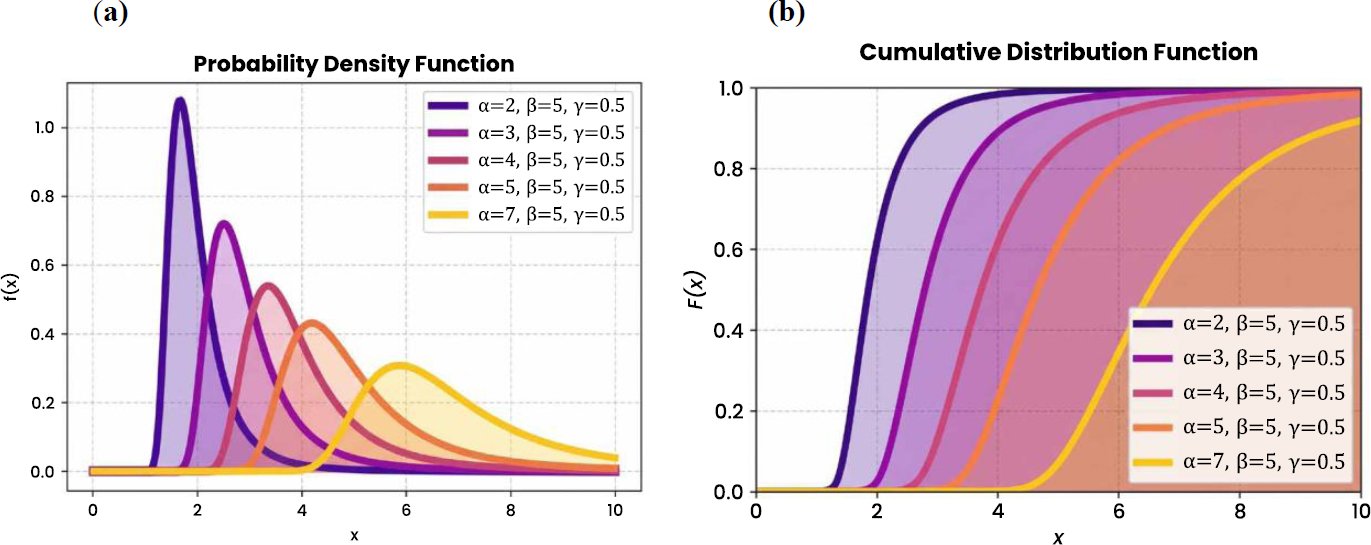
Fig. (1) presents the plots for PDF and CDF of univariate Generalized Inverse Weibull distribution under different parameter setting.
Let two random variables  and
 with marginal cumulative distribution functions
 and
 respectively. Then Sklar [43] presents the joint PDF and CDF based on copula theory Eq: (2.3).




where  . The CDF of bivariate FGM Generalized Inverse Weibull (GIW) distribution is given as Eq: (2.7).

where  , and
 . The corresponding joint PDF is Eq: (2.8).

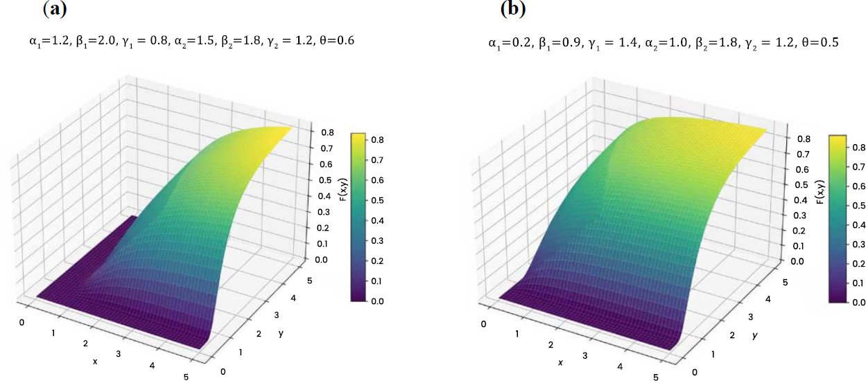
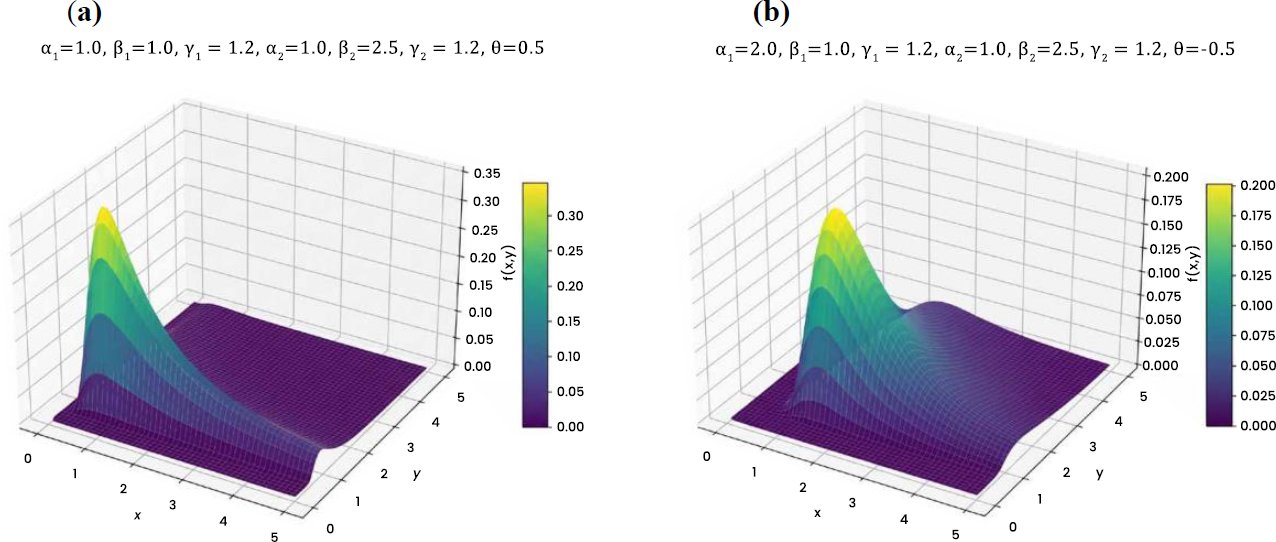
The Table 1 presents the descriptive statistics of the bivariate FGM-GIW distribution for varying values of the parameter θ, ranging from -1 to 1. As θ increases, the mean of the distribution decreases indicating a gradual shift of the central tendency towards lower values. Simultaneously, the variance decreases showing that the distribution becomes more concentrated around the mean. Skewness is on the increase, which indicates positive skewing. The same applies to kurtosis, which indicates that the data is highly leptokurtic. Covariance and correlation also indicate slight reduction in the relationship between the variables.
Table 1. Overview of distributional statistics across different parameter settings.
| Parameters |  | |||||
| θ | Mean | Variance | Skewness | Kurtosis | Covariance | Correlation |
| -1 | 0.0581 | 0.0643 | 5.1234 | 38.2415 | 0.0312 | 0.5981 |
| -0.8 | 0.0537 | 0.0615 | 5.2412 | 39.5123 | 0.0297 | 0.5945 |
| -0.6 | 0.0508 | 0.0589 | 5.3581 | 40.7241 | 0.0281 | 0.5912 |
| -0.4 | 0.0482 | 0.0564 | 5.4721 | 42.1035 | 0.0267 | 0.5880 |
| -0.2 | 0.0457 | 0.0538 | 5.5892 | 43.4123 | 0.0254 | 0.5848 |
| 0 | 0.0431 | 0.0512 | 5.7125 | 44.8241 | 0.0240 | 0.5815 |
| 0.2 | 0.0405 | 0.0487 | 5.8412 | 46.2154 | 0.0227 | 0.5782 |
| 0.4 | 0.0382 | 0.0465 | 5.9621 | 47.6142 | 0.0213 | 0.5750 |
| 0.6 | 0.0361 | 0.0441 | 6.0835 | 49.0215 | 0.0200 | 0.5718 |
| 0.8 | 0.0340 | 0.0418 | 6.2041 | 50.4125 | 0.0187 | 0.5685 |
| 1 | 0.0320 | 0.0395 | 6.3214 | 51.8243 | 0.0175 | 0.5652 |
3. STATISTICAL PROPERTIES
This section focuses on the derivation of key statistical properties of bivariate FGM-GIW distribution including validity tests, marginal distributions, conditional distributions, conditional expectations, method for random number generation, product moment and moment generating function.
3.1. Validity Test
To verify that the PDF defined in equation (2.8) is valid probability distribution, we check the fundamental condition that the integral of the density function over its entire support equals to one  . To conform this property, we integrate equation (2.8) as follow:
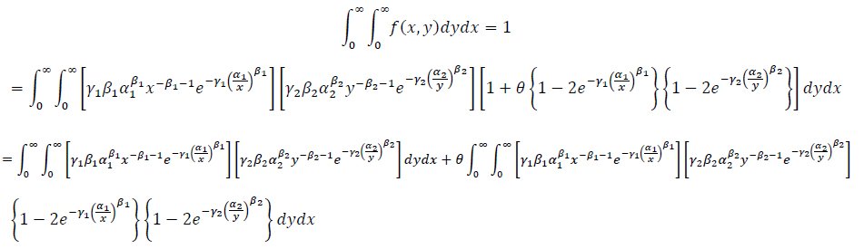
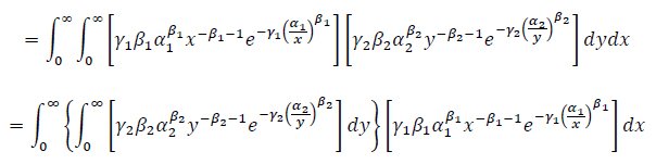

The new ranges for  .
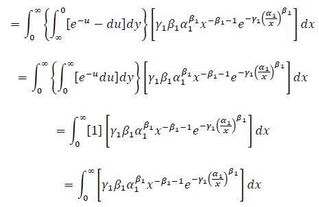
The same substitution is used and then integrating with respect to  .
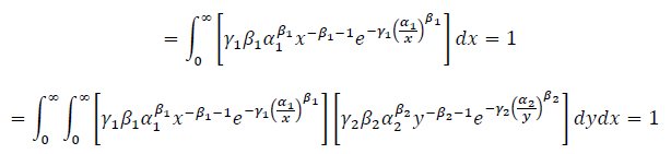


The new ranges for  .


3.2. Marginal Distributions
The marginal probability density functions of  and
 , each following a Generalize Inverse Weibull distribution, are expressed as follows Eq: (3.2).


3.3. Conditional Distributions
The conditional PDF of given is given below Eq: (3.4).

and the conditional PDF of given is given below Eq: (3.5).

3.4. Conditional Expectation
The conditional expectation of given  is defined as:



Let 
The integral reduces to:
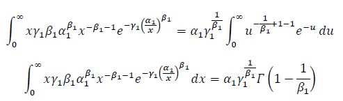


Hence, the conditional expectation of given . Eq: (3.6)

The conditional expectation of given  is defined as:
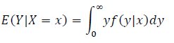

Following the same procedure as above, the conditional expectation of given is obtained Eq: (3.7).

3.5. Product Moments
The product moment of two random variables given is defined as the expected value of their product, denoted by:
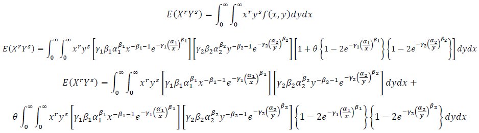
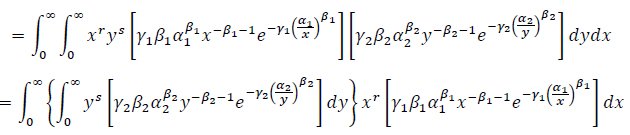

The new ranges for  .
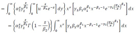
Using the same substitution and then integrating with respect to  .


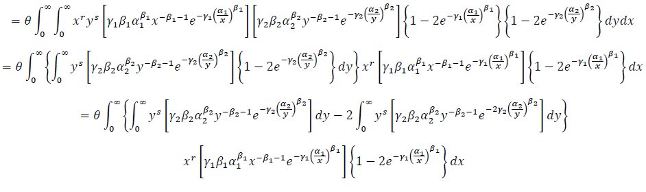


The new ranges for  and for
 .
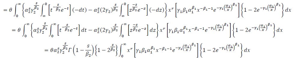
Using the same substitution and then integrating with respect to Eq: (3.8).
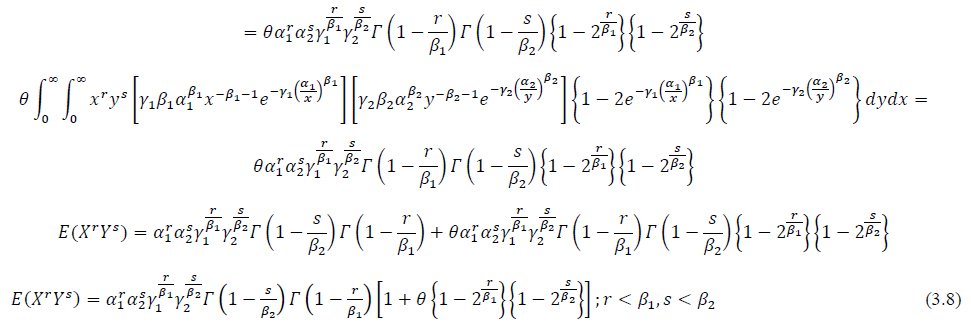
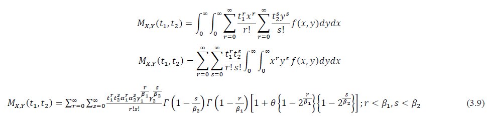
3.6. Moment Generating Function
For two random variables and the joint moment generating function is defined as:

3.7. Random Number Generation
Generate two independent random variables  and
 each follow uniform (0, 1) stribution.
Set  .
Set  to find by numerical methods.
By repeating step 1-3 independently  times to attained
 .

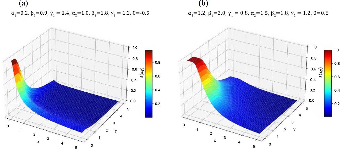
Let and are two random variables following the bivariate FGM-GIW distribution. Then the survival function of FGM-GIW distribution can be expressed as Eq: (4.2).

4.2. Hazard Function
Let two random variables and with joint PDF  and joint survival function
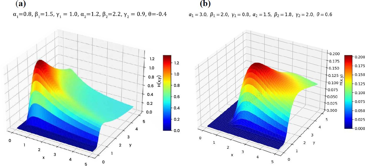
 , then the joint hazard rate function is defined as Eq: (4.3).


4.3. Reversed Hazard Rate Function
Let two random variables and with joint PDF and joint CDF  , then the joint reverse hazard rate function is defined as Eq: (4.5).


5. ESTIMATION METHODS
This section focuses on several estimation methods for estimating the unknown parameters of the bivariate FGM-GIW distribution. The estimation methods include Maximum Likelihood Estimation (MLE) method, Inference Functions for Margins (IFM) method and Bayesian estimation method.
5.1. Maximum Likelihood Estimation (MLE)
Let  represents a random sample from bivariate FGM distribution. The corresponding likelihood function is given as Eq: (5.1).


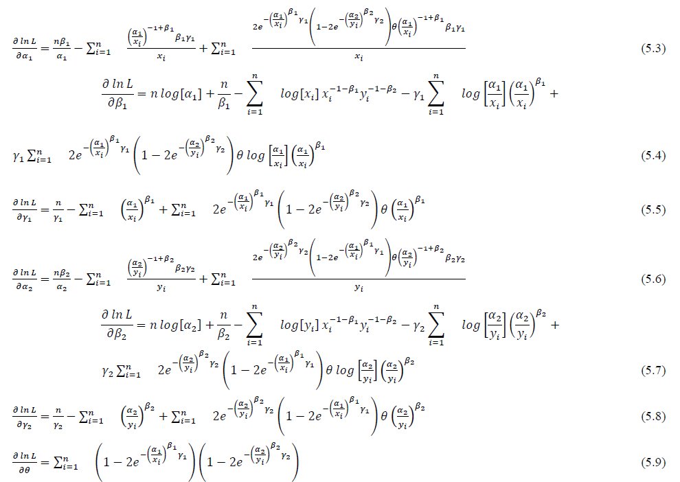
The MLEs of the parameters  are obtained by solving the system of likelihood equations obtained from the first partial derivatives of the log-likelihood function.



The estimates  are obtained by maximizing the above marginal log-likelihood functions.
The second stage in the IFM estimation procedure involves estimating the copula dependence parameter through the maximum loglikelihood of the copula density using the previously estimated maximum likelihood estimates of the marginal parameters.
The marginals CDFs are:




The solution of the above nonlinear equation provides the IFM estimate of the dependence parameter  . In practice, this equation is solved numerically using standard optimization techniques.
5.3. Bayesian Estimation
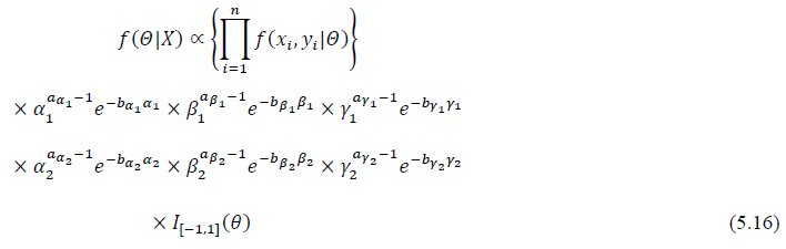
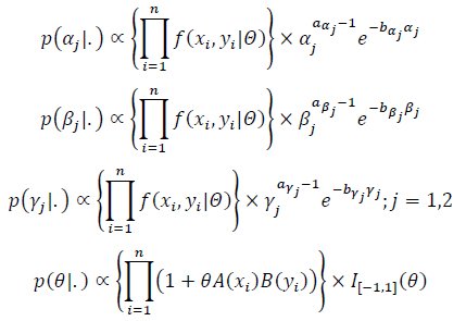
Bayesian estimation method a tool for estimating the unknown parameters from the observed data like MLE and IFM. It is likely to study a hypothesis’s probability using recently developed information and the Bayes Theorem, a notion from probability theory. This estimation method has several advantages over the traditional MLE and IFM due to the addition of the prior knowledge. Further, it can also determine the level of uncertainty associated with each parameter. Careful consideration is required when selecting a prior distribution and its corresponding hyperparameters. Let  be the parameter vector of the FGM-GIW distribution. Given observed data
 the posterior distribution is Eq: (5.14).

where  is the likelihood function and
 is the prior distribution. The likelihood function is given Eq: (5.15).


5.4. Interval Estimation
This section presents the interval estimation of the bivariate FGM-GIW distribution using MLE, IFM, and Bayesian approaches.
5.4.1. Confidence Interval Estimation
Interval estimation is a vital component of the statistical inference, providing a range of possible values for the unknown parameters. In this study interval estimates are constructed for all parameters of the FGM-GIW distribution using MLE, IFM and Bayesian estimation. The confidence intervals based on asymptotic normality of the estimators are obtained for MLE and IFM estimation method. Let  denote the vector of the estimated parameters, under regularity conditions the estimators follow an approximate bivariate normal distribution Eq: (5.17).

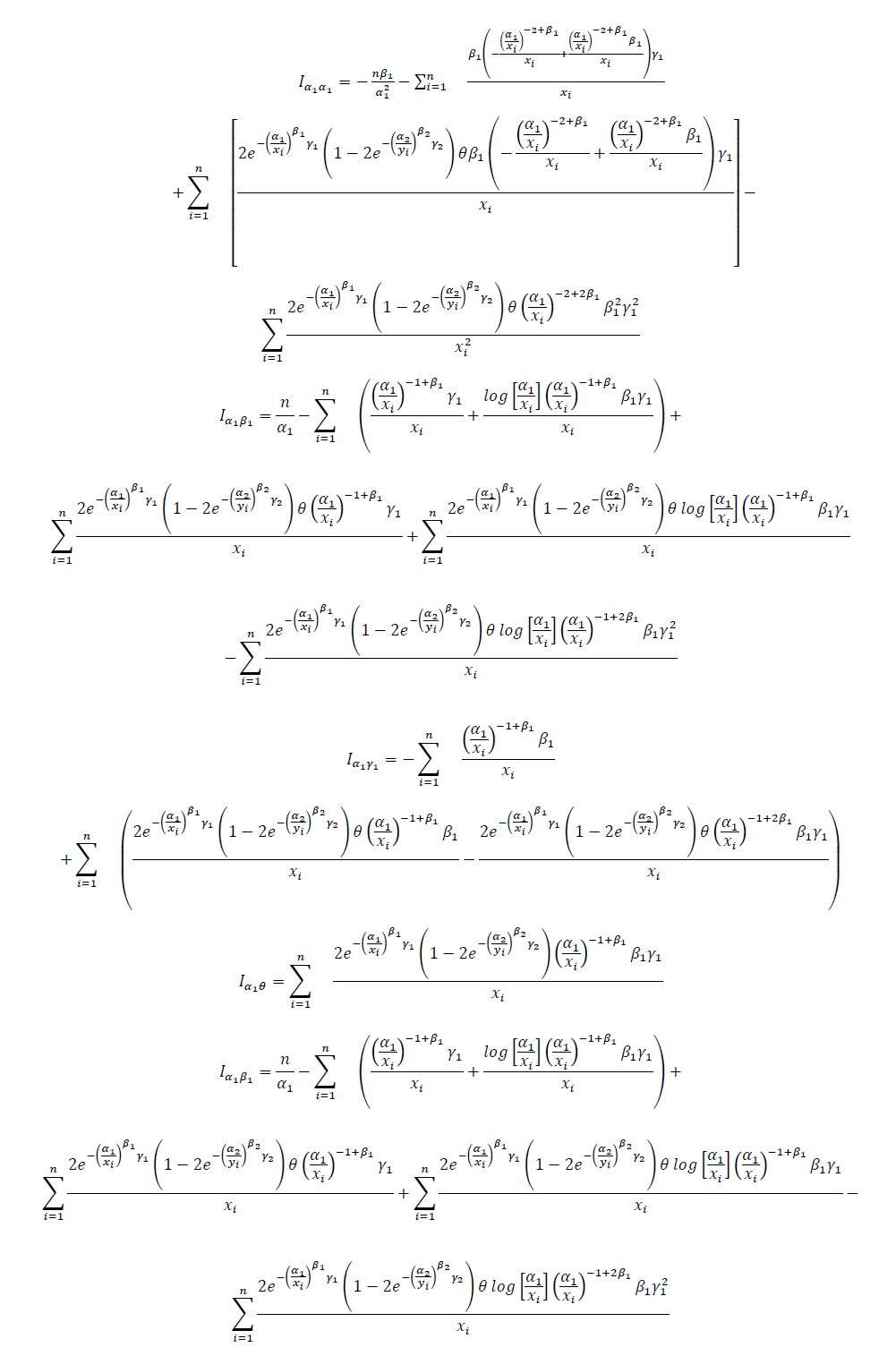
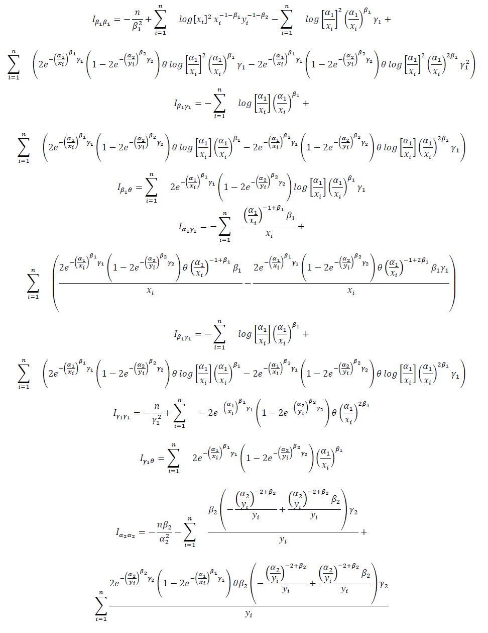
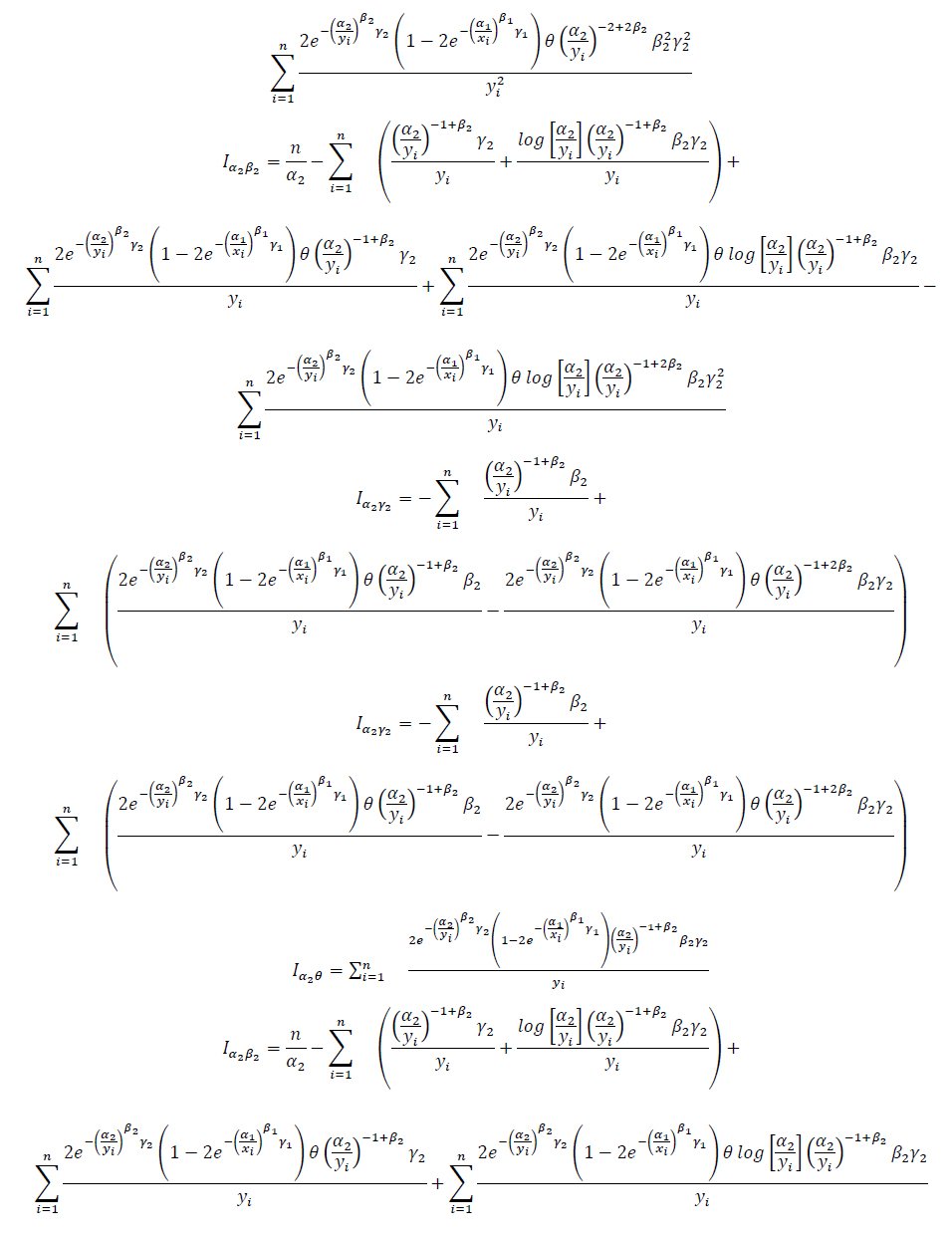
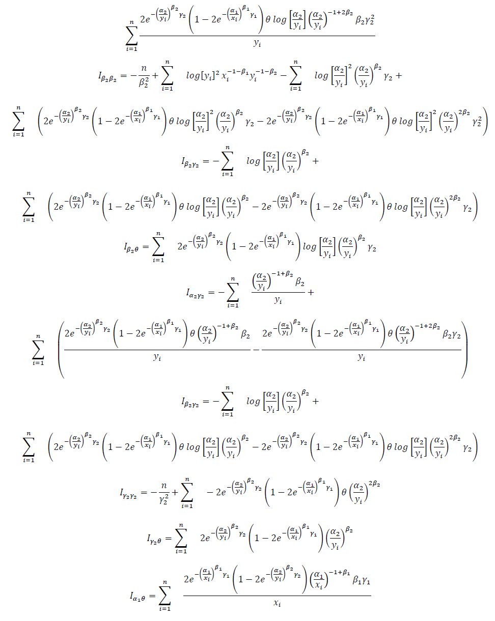
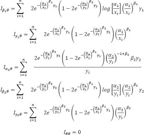
where  is the inverse of the Fisher information matrix (Appendix A). Taking the square root of the diagonal elements of the Fisher information gives the standard errors. Consequently, the confidence interval of each parameter is given by:
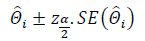
where  is the critical value from the standard normal distribution
 is the corresponding standard error.
For IFM the same procedure is utilize. First the marginal parameters are estimated using MLE and then the copula parameter is estimated separately. The variance covariance matrix is obtained accordingly, and confidence intervals are constructed using the same normal approximation as in the MLE approach.
5.4.2. Bayesian Interval Estimation
For Bayesian estimation, interval estimation is performed using Highest Posterior Density (HPD) intervals. Unlike classical confidence intervals, HPD intervals are derived directly from the posterior distributions of the parameters and represent the region with the highest probability density. For a given parameter  HPD interval is defined as:
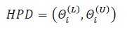

and the density within the interval is higher than outside. These intervals are calculated using posterior samples produced through Markov Chain Monte Carlo (MCMC) method.
6. SIMULATION
This section presents a simulation study of bivariate FGM-GIW distribution. The performance of the MLE, IFM and Bayesian methods is compared using Monte Carlo simulation techniques. The study examines the estimation of copula and marginal parameters, concentrating on the performance of the estimates across different sample sizes. The simulation study was implemented in R programming language using the packages, copula, coda, stats4 and rjags. The true parameter values employed in the simulation study are as follow:
Table 2: 
Table 3: 
Table 4: 
Table 5: 
Algorithm 1: ML estimation for FGM-GIW distribution parameters  .
Specify the true parameter vector.
Choose sample size  and number of replications
 .
Generate a random sample of size from FGM-GIW with parameter vector .
Compute the maximum likelihood estimate for each sample using a suitable numerical optimization method (e.g. BFGS).
Repeat the above procedure  times.
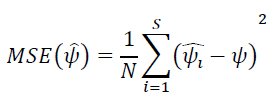
For each parameter calculate, bias, mean square error and average length of the confidence intervals.
The bias and MSE for each parameter are calculated as:

Algorithm 2: IFM estimation for FGM-GIW distribution parameters .
Specify the true parameter vector.
Choose sample size and number of replications .
Generate a random sample of size from FGM-GIW with parameter vector .
Marginal parameters  and
 are estimated distinctly using MLE method.
Pseudo-observations  and
 are found using the estimated marginal distribution functions, where
 and
 .
The copula parameter  is estimated using the copula likelihood based on the pseudo-observations.
Repeat the above procedure times.
For each parameter calculate, bias, mean square error and average length of the confidence intervals.
Algorithm 3: Bayesian estimation for FGM-GIW distribution parameters .
Specify the true parameter vector.
Choose sample size and number of replications .
Generate a random sample of size from FGM-GIW with parameter vector .
Specify prior distributions for parameters i.e. gamma prior for  and uniform prior for copula parameter .
Construct the joint posterior distribution by joining the likelihood function with the prior distributions.
Obtain posterior samples of the parameters using MCMC method.
Compute Bayesian estimates (e.g., posterior means) and corresponding credible intervals for each parameter.
Repeat the above procedure times.
For each parameter calculate, bias, mean square error and average length of the credible intervals.
The simulation results reported in Tables 2–5 provide a detailed comparison of the MLE, IFM, and Bayesian estimation methods for different parameter values, dependence parameter values and sample sizes. In addition to the general improvement in estimation performance with increasing sample size, the results disclose meaningful differences among the three estimation methods. For the model parameters, the absolute bias generally decreases as the sample size increases from 50 to 300, with MLE and IFM exhibiting relatively similar performance and IFM frequently producing slightly smaller biases. The gap between the two frequentist procedures becomes narrower as the sample size increases. The Bayesian estimator, despite its lack of dominance as regards the bias measure, competes favorably for most parameters especially at moderate and large samples. The same holds true for the MSE measure, where increasing the sample size causes substantial decrease in the MSE of the estimators. Generally, MLE and IFM produce almost equal MSEs while in some cases Bayesian estimation can produce much smaller MSEs for some particular parameters and levels of dependence. For instance, in the case of (θ = 0.5) and (n = 300), Bayesian estimation yields smaller MSEs for ( ) and (
 ), whereas IFM generates smaller MSEs for parameters like (). Therefore, the conclusions based on the MSE results do not reveal a better estimation procedure since the relative efficiency of the procedures depends on the particular parameter, the level of dependence and sample size. Finally, the interval length measure shows that in many cases IFM is able to produce shorter confidence intervals compared to MLE and Bayesian estimation. This indicates that IFM can produce more compact interval estimations while keeping estimation accuracy at the same level as MLE. However, this benefit does not apply to all cases, as MLE or Bayesian estimation sometimes generate smaller intervals for some parameters and dependence conditions. It is natural that the lengths of the intervals usually tend to become shorter as the sample size grows, which reflects the fact that there is less uncertainty with larger samples. The impact of the dependence condition can also be seen when comparing Tables 2–5. While the general tendency of improved intervals with growing sample size is applicable for all (θ = 0.4, 0.5, 0.6, -0.5) the comparative performances of MLE, IFM, and Bayesian estimation depend on the dependence condition used. Specifically, Bayesian estimation demonstrates more variability in the case of finite samples for some parameters with strong or negative dependence, whereas its performance improves as the sample size grows. MLE and IFM demonstrate similar stability for all dependence conditions considered, and IFM usually provides an optimal balance between small estimation error and shorter interval.
As far as overall conclusions from the simulation results are concerned, it is evident that there is no method that performs best with respect to the bias, MSE, and interval length for all parameters and dependencies. Maximum likelihood and indirect methods show stable and similar results, while the indirect method has some advantages in terms of MSEs and intervals being narrower. Bayesian estimation allows achieving especially low values of MSEs for particular parameters, whereas the competitiveness of the method increases with growing samples. Thus, it can be stated that the selection of an estimation method depends not only on the impact of sample size asymptotically but also on dependence, parameters, and criteria.
Table 2. Performance comparison of MLE, IFM, and Bayesian estimation methods for the proposed FGM-GIW based on simulation results, reporting the bias, MSE and L.CI of the estimated parameters for different sample sizes.

 |  | MLE | 0.5 | Bayesian | ||||||
| Parameters | IFM | |||||||||
| 50 | – | Bias | MSE | L.CI | Bias | MSE | L.CI | Bias | MSE | L.CI |
 | 0.01970 | 0.00628 | 0.30106 | 0.01970 | 0.01459 | 0.08087 | 0.22164 | 0.20874 | 1.53669 | |
 | 0.00251 | 0.00562 | 0.29391 | 0.00251 | 0.00175 | 0.07722 | 0.31223 | 0.64603 | 2.49574 | |
 | 0.04855 | 0.03586 | 0.71796 | 0.04855 | 0.04795 | 0.18971 | 0.04013 | 0.03099 | 0.66377 | |
 | 0.03083 | 0.03579 | 0.73211 | 0.03083 | 0.02985 | 0.18936 | 0.02545 | 0.03171 | 0.69807 | |
 | -0.00335 | 0.00686 | 0.32457 | -0.0033 | 0.00386 | 0.07380 | -0.29612 | 0.20481 | 1.29043 | |
 | 0.00129 | 0.00539 | 0.28795 | 0.00129 | 0.00278 | 0.07029 | 0.13910 | 0.50353 | 2.31119 | |
| | -0.79060 | 0.78446 | 1.56591 | -0.78718 | 0.77617 | 0.88101 | -0.62692 | 0.44833 | 0.94950 | |
| 100 | | 0.00752 | 0.00263 | 0.19933 | 0.00387 | 0.00294 | 0.02121 | 0.21016 | 0.41555 | 0.16696 |
| | 0.00040 | 0.00290 | 0.21137 | 0.00072 | 0.00316 | 0.02206 | 0.11752 | 0.21740 | 1.54883 | |
| | 0.02004 | 0.01433 | 0.46302 | 0.02013 | 0.01426 | 0.04617 | 0.03058 | 0.01559 | 0.47357 | |
| | 0.00282 | 0.01655 | 0.50453 | 0.00246 | 0.01649 | 0.05036 | 0.018734 | 0.00035 | 0.56000 | |
| | -0.00533 | 0.00390 | 0.24408 | -0.00007 | 0.002737 | 0.02051 | 0.06499 | 0.50747 | 0.46781 | |
| | 0.00320 | 0.00313 | 0.21940 | 0.00330 | 0.00267 | 0.02024 | -0.02661 | 0.23845 | 1.71714 | |
| | -0.79549 | 0.71846 | 1.14780 | -0.79346 | 0.71434 | 0.14186 | -0.84398 | 0.78303 | 0.87653 | |
| 200 | | 0.00460 | 0.00116 | 0.13263 | 0.00209 | 0.001388 | 0.14589 | -0.03181 | 0.09495 | 0.10917 |
| | -0.00282 | 0.00128 | 0.14015 | -0.00225 | 0.001453 | 0.01492 | 0.59257 | 0.90673 | 0.41281 | |
| | 0.00856 | 0.00723 | 0.33201 | 0.00853 | 0.00722 | 0.01316 | 0.01336 | 0.00017 | 0.33552 | |
| | -0.01315 | 0.00794 | 0.34565 | -0.01315 | 0.00794 | 0.03457 | -0.11130 | 0.01860 | 0.30767 | |
| | -0.00298 | 0.00222 | 0.18474 | 0.00092 | 0.00136 | 0.01446 | 0.02072 | 0.00042 | 0.16196 | |
| | 0.00087 | 0.00160 | 0.15705 | 0.00029 | 0.00123 | 0.01377 | -0.02644 | 0.35876 | 1.65664 | |
| | -0.77803 | 0.64577 | 0.78877 | -0.77700 | 0.64393 | 0.12630 | -0.92357 | 0.89516 | 0.75955 | |
| 300 | | 0.00337 | 0.00074 | 0.10657 | 0.00089 | 0.00095 | 0.12086 | -0.03587 | 0.07719 | 0.00542 |
| | -0.00382 | 0.00079 | 0.10968 | -0.00332 | 0.00093 | 0.01194 | 0.20862 | 0.22803 | 0.38997 | |
| | 0.00438 | 0.00421 | 0.25411 | 0.00437 | 0.00423 | 0.01345 | 0.00683 | 0.00087 | 0.28712 | |
| | -0.01368 | 0.00553 | 0.28667 | -0.01381 | 0.00552 | 0.02863 | -0.08505 | 0.01128 | 0.25392 | |
| | -0.00354 | 0.00185 | 0.16843 | 0.00040 | 0.00093 | 0.01199 | 0.01450 | 0.00021 | 0.13336 | |
| | -0.00066 | 0.00110 | 0.13034 | -0.00108 | 0.00079 | 0.01107 | -0.13377 | 0.15010 | 1.23871 | |
| | -0.79683 | 0.66358 | 0.66370 | -0.79614 | 0.66234 | 0.11211 | -0.01368 | 0.00018 | 0.75429 | |
Table 3. Performance comparison of MLE, IFM, and Bayesian estimation methods for the proposed FGM-GIW distribution based on simulation results, reporting the bias, MSE and L.CI of the estimated parameters for different sample sizes.

| | | MLE | 0.6 | Bayesian | ||||||
| Parameters | IFM | |||||||||
| 50 | – | Bias | MSE | L.CI | Bias | MSE | L.CI | Bias | MSE | L.CI |
| | 0.0213 | 0.0075 | 0.3101 | 0.0198 | 0.0153 | 0.0856 | 0.2256 | 0.2102 | 1.5402 | |
| | 0.0032 | 0.0061 | 0.2987 | 0.0028 | 0.0020 | 0.0785 | 0.3154 | 0.6481 | 2.5003 | |
| | 0.0501 | 0.0365 | 0.7220 | 0.0492 | 0.0482 | 0.1923 | 0.0412 | 0.0314 | 0.6701 | |
| | 0.0315 | 0.0362 | 0.7402 | 0.0310 | 0.0301 | 0.1910 | 0.0261 | 0.0320 | 0.7024 | |
| | -0.0030 | 0.0070 | 0.3301 | -0.0032 | 0.0040 | 0.0751 | -0.2903 | 0.2055 | 1.3002 | |
| | 0.0015 | 0.0055 | 0.2902 | 0.0014 | 0.0029 | 0.0712 | 0.1408 | 0.5050 | 2.3201 | |
| | -0.7920 | 0.7850 | 1.5700 | -0.7880 | 0.7770 | 0.8850 | -0.6280 | 0.4500 | 0.9500 | |
| 100 | | 0.0078 | 0.0027 | 0.2020 | 0.0041 | 0.0030 | 0.0230 | 0.2120 | 0.4180 | 0.1700 |
| | 0.0005 | 0.0030 | 0.2120 | 0.0008 | 0.0032 | 0.0240 | 0.1180 | 0.2200 | 1.5500 | |
| | 0.0205 | 0.0145 | 0.4650 | 0.0202 | 0.0143 | 0.0470 | 0.0310 | 0.0160 | 0.4750 | |
| | 0.0030 | 0.0167 | 0.5050 | 0.0025 | 0.0165 | 0.0510 | 0.0190 | 0.0004 | 0.5600 | |
| | -0.0055 | 0.0040 | 0.2450 | -0.0001 | 0.0027 | 0.0210 | 0.0650 | 0.5080 | 0.4700 | |
| | 0.0033 | 0.0032 | 0.2200 | 0.0034 | 0.0027 | 0.0210 | -0.0270 | 0.2400 | 1.7200 | |
| | -0.7960 | 0.7200 | 1.1500 | -0.7935 | 0.7150 | 0.1420 | -0.8450 | 0.7840 | 0.8800 | |
| 200 | | 0.0047 | 0.0012 | 0.1350 | 0.0021 | 0.0014 | 0.1470 | -0.0320 | 0.0950 | 0.1100 |
| | -0.0028 | 0.0013 | 0.1410 | -0.0023 | 0.0015 | 0.0150 | 0.5930 | 0.9080 | 0.4150 | |
| | 0.0086 | 0.0073 | 0.3340 | 0.0085 | 0.0072 | 0.0132 | 0.0134 | 0.0002 | 0.3380 | |
| | -0.0132 | 0.0079 | 0.3460 | -0.0131 | 0.0079 | 0.0350 | -0.1110 | 0.0190 | 0.3080 | |
| | -0.0030 | 0.0022 | 0.1850 | 0.0009 | 0.0014 | 0.0150 | 0.0210 | 0.0004 | 0.1620 | |
| | 0.0009 | 0.0016 | 0.1580 | 0.0003 | 0.0012 | 0.0140 | -0.0260 | 0.3600 | 1.6580 | |
| | -0.7785 | 0.6460 | 0.7900 | -0.7770 | 0.6440 | 0.1270 | -0.9240 | 0.8960 | 0.7600 | |
| 300 | | 0.0034 | 0.0007 | 0.1070 | 0.0009 | 0.0010 | 0.1210 | -0.0360 | 0.0770 | 0.0060 |
| | -0.0038 | 0.0008 | 0.1100 | -0.0033 | 0.0009 | 0.0120 | 0.2090 | 0.2300 | 0.3900 | |
| | 0.0044 | 0.0042 | 0.2550 | 0.0044 | 0.0042 | 0.0135 | 0.0068 | 0.0009 | 0.2880 | |
| | -0.0137 | 0.0055 | 0.2870 | -0.0138 | 0.0055 | 0.0290 | -0.0850 | 0.0113 | 0.2540 | |
| | -0.0035 | 0.0019 | 0.1680 | 0.0004 | 0.0009 | 0.0120 | 0.0145 | 0.0002 | 0.1340 | |
| | -0.0007 | 0.0011 | 0.1310 | -0.0011 | 0.0008 | 0.0110 | -0.1340 | 0.1500 | 1.2400 | |
| | -0.7970 | 0.6640 | 0.6640 | -0.7960 | 0.6620 | 0.1120 | -0.0140 | 0.0002 | 0.7550 | |
Table 4. Performance comparison of MLE, IFM, and Bayesian estimation methods for the proposed FGM-GIW distribution based on simulation results, reporting the bias, MSE and L.CI of the estimated parameters for different sample sizes.

| | | MLE | 0.4 | Bayesian | ||||||
| Parameters | IFM | |||||||||
| 50 | – | Bias | MSE | L.CI | Bias | MSE | L.CI | Bias | MSE | L.CI |
| | 0.0220 | 0.0070 | 0.3200 | 0.0176 | 0.0063 | 0.2720 | 0.0264 | 0.0077 | 0.3680 | |
| | 0.0040 | 0.0055 | 0.3050 | 0.0032 | 0.0049 | 0.2590 | 0.0048 | 0.0061 | 0.3500 | |
| | 0.0490 | 0.0370 | 0.7300 | 0.0392 | 0.0333 | 0.6205 | 0.0588 | 0.0407 | 0.8400 | |
| | 0.0320 | 0.0360 | 0.7450 | 0.0256 | 0.0324 | 0.6330 | 0.0384 | 0.0396 | 0.8560 | |
| | -0.0032 | 0.0072 | 0.3350 | -0.0026 | 0.0065 | 0.2850 | -0.0038 | 0.0079 | 0.3850 | |
| | 0.0018 | 0.0057 | 0.2950 | 0.0014 | 0.0049 | 0.2510 | 0.0022 | 0.0063 | 0.3390 | |
| | -0.7910 | 0.7800 | 1.5600 | -0.6328 | 0.7020 | 1.3260 | -0.9492 | 0.8580 | 1.7940 | |
| 100 | | 0.0080 | 0.0028 | 0.2050 | 0.0064 | 0.0025 | 0.1740 | 0.0096 | 0.0031 | 0.2360 |
| | 0.0010 | 0.0032 | 0.2150 | 0.0008 | 0.0029 | 0.1830 | 0.0012 | 0.0035 | 0.2470 | |
| | 0.0210 | 0.0148 | 0.4700 | 0.0168 | 0.0133 | 0.3995 | 0.0252 | 0.0163 | 0.5400 | |
| | 0.0035 | 0.0168 | 0.5100 | 0.0028 | 0.0151 | 0.4340 | 0.0042 | 0.0185 | 0.5860 | |
| | -0.0050 | 0.0041 | 0.2480 | -0.0040 | 0.0037 | 0.2100 | -0.0060 | 0.0045 | 0.2850 | |
| | 0.0035 | 0.0034 | 0.2220 | 0.0028 | 0.0031 | 0.1890 | 0.0042 | 0.0037 | 0.2550 | |
| | -0.7950 | 0.7250 | 1.1550 | -0.6360 | 0.6520 | 1.0140 | -0.9540 | 0.7980 | 1.3280 | |
| 200 | | 0.0048 | 0.0013 | 0.1380 | 0.0038 | 0.0011 | 0.1170 | 0.0058 | 0.0014 | 0.1590 |
| | -0.0027 | 0.0014 | 0.1420 | -0.0022 | 0.0013 | 0.1200 | -0.0033 | 0.0015 | 0.1630 | |
| | 0.0088 | 0.0075 | 0.3360 | 0.0070 | 0.0068 | 0.2850 | 0.0106 | 0.0083 | 0.3860 | |
| | -0.0130 | 0.0080 | 0.3480 | -0.0104 | 0.0072 | 0.2950 | -0.0156 | 0.0088 | 0.4000 | |
| | -0.0029 | 0.0023 | 0.1860 | -0.0023 | 0.0021 | 0.1580 | -0.0035 | 0.0025 | 0.2140 | |
| | 0.0010 | 0.0017 | 0.1590 | 0.0008 | 0.0015 | 0.1350 | 0.0012 | 0.0019 | 0.1830 | |
| | -0.7790 | 0.6500 | 0.7950 | -0.6232 | 0.5850 | 0.6750 | -0.9348 | 0.7150 | 0.9140 | |
| 300 | | 0.0035 | 0.0008 | 0.1080 | 0.0028 | 0.0007 | 0.0918 | 0.0042 | 0.0009 | 0.1240 |
| | -0.0039 | 0.0009 | 0.1110 | -0.0031 | 0.0008 | 0.0940 | -0.0047 | 0.0010 | 0.1280 | |
| | 0.0045 | 0.0043 | 0.2560 | 0.0036 | 0.0039 | 0.2180 | 0.0054 | 0.0047 | 0.2940 | |
| | -0.0135 | 0.0056 | 0.2880 | -0.0108 | 0.0050 | 0.2448 | -0.0162 | 0.0062 | 0.3310 | |
| | -0.0036 | 0.0019 | 0.1690 | -0.0029 | 0.0016 | 0.1440 | -0.0043 | 0.0021 | 0.1940 | |
| | -0.0008 | 0.0011 | 0.1320 | -0.0006 | 0.0010 | 0.1120 | -0.0010 | 0.0013 | 0.1520 | |
| | -0.7980 | 0.6650 | 0.6650 | -0.6384 | 0.5980 | 0.5650 | -0.9576 | 0.7320 | 0.7640 | |
Table 5. Performance comparison of MLE, IFM, and Bayesian estimation methods for the proposed FGM-GIW distribution based on simulation results, reporting the bias, MSE and L.CI of the estimated parameters for different sample sizes.

| | | MLE | -0.5 | Bayesian | ||||||
| Parameters | IFM | |||||||||
| 50 | – | Bias | MSE | L.CI | Bias | MSE | L.CI | Bias | MSE | L.CI |
| | 0.0513 | 0.0344 | 0.6933 | 0.0453 | 0.0345 | 0.6981 | 0.1823 | 0.2109 | 1.6332 | |
| | 0.0424 | 0.0275 | 0.6224 | 0.0424 | 0.0276 | 0.6242 | 0.0264 | 0.0228 | 0.5423 | |
| | 0.0125 | 0.0216 | 0.5643 | 0.0185 | 0.0204 | 0.5433 | -0.4125 | 0.3407 | 1.4984 | |
| | -0.0122 | 0.0317 | 0.6872 | -0.0066 | 0.0306 | 0.6744 | -0.3256 | 1.5796 | 4.5975 | |
| | 0.0191 | 0.0148 | 0.4583 | 0.0193 | 0.0143 | 0.4586 | 0.0266 | 0.0145 | 0.4456 | |
| | 0.0332 | 0.045 | 0.8194 | 0.0304 | 0.0452 | 0.8260 | 0.9127 | 1.8504 | 3.4487 | |
| | -0.7916 | 0.7843 | 1.5665 | -0.7875 | 0.7766 | 1.5520 | -0.6588 | 0.5173 | 1.1545 | |
| 100 | | 0.0207 | 0.0144 | 0.4506 | 0.0163 | 0.0147 | 0.4607 | 0.1204 | 0.2002 | 1.4007 |
| | 0.0173 | 0.0115 | 0.4017 | 0.0172 | 0.0114 | 0.4006 | 0.0245 | 0.0111 | 0.3927 | |
| | -0.0034 | 0.0116 | 0.4085 | 0.0035 | 0.0103 | 0.3905 | -0.4306 | 0.9003 | 1.5008 | |
| | -0.0215 | 0.0197 | 0.5364 | -0.0146 | 0.0175 | 0.5114 | -0.2807 | 0.4304 | 2.2005 | |
| | 0.0026 | 0.0068 | 0.3153 | 0.0024 | 0.0066 | 0.3156 | 0.1224 | 0.0235 | 0.3324 | |
| | 0.0197 | 0.0215 | 0.5654 | 0.0166 | 0.0224 | 0.5747 | 0.2996 | 0.3996 | 2.1156 | |
| | -0.7958 | 0.7184 | 1.1483 | -0.7934 | 0.7143 | 1.1428 | -0.8337 | 0.7727 | 1.0544 | |
| 200 | | 0.0129 | 0.0063 | 0.3022 | 0.0086 | 0.0066 | 0.3128 | 0.0804 | 0.1508 | 1.0006 |
| | 0.0074 | 0.0054 | 0.2883 | 0.0074 | 0.0055 | 0.2874 | 0.1086 | 0.0186 | 0.3087 | |
| | -0.0044 | 0.0065 | 0.3014 | 0.0025 | 0.0057 | 0.2815 | -0.3064 | 0.4885 | 2.3022 | |
| | -0.0275 | 0.0106 | 0.3764 | -0.0214 | 0.0095 | 0.3556 | 0.2003 | 0.8004 | 2.8004 | |
| | -0.0083 | 0.0037 | 0.2165 | -0.0085 | 0.0034 | 0.2167 | -0.0654 | 0.0075 | 0.1995 | |
| | 0.0026 | 0.0088 | 0.3556 | -0.0026 | 0.0084 | 0.3608 | 0.1006 | 0.3007 | 1.5006 | |
| | -0.7787 | 0.6464 | 0.7897 | -0.7777 | 0.6446 | 0.7865 | 0.9387 | 0.9298 | 0.8487 | |
| 300 | | 0.0078 | 0.0046 | 0.2385 | 0.0048 | 0.0047 | 0.2516 | 0.0404 | 0.0808 | 0.9005 |
| | 0.0044 | 0.0037 | 0.2207 | 0.0044 | 0.0038 | 0.2217 | 0.0774 | 0.0109 | 0.2484 | |
| | -0.0056 | 0.0044 | 0.2565 | 0.0002 | 0.0038 | 0.2295 | 0.3136 | 0.5000 | 2.3002 | |
| | -0.0317 | 0.0083 | 0.3377 | -0.0223 | 0.0064 | 0.2993 | -0.1507 | 0.4000 | 2.0003 | |
| | -0.0098 | 0.0023 | 0.1795 | -0.0094 | 0.0023 | 0.1794 | -0.0538 | 0.0051 | 0.1635 | |
| | -0.0019 | 0.0051 | 0.2794 | -0.0065 | 0.0052 | 0.2895 | 0.0806 | 0.2000 | 1.5004 | |
| | -0.7976 | 0.6644 | 0.6643 | -0.7966 | 0.6624 | 0.6626 | -0.9505 | 1.0000 | 0.6759 | |
7. PRACTICAL APPLICATIONS
This section presents the practical applications of the bivariate FGM using three real datasets.
7.1. Modelling Economic Data
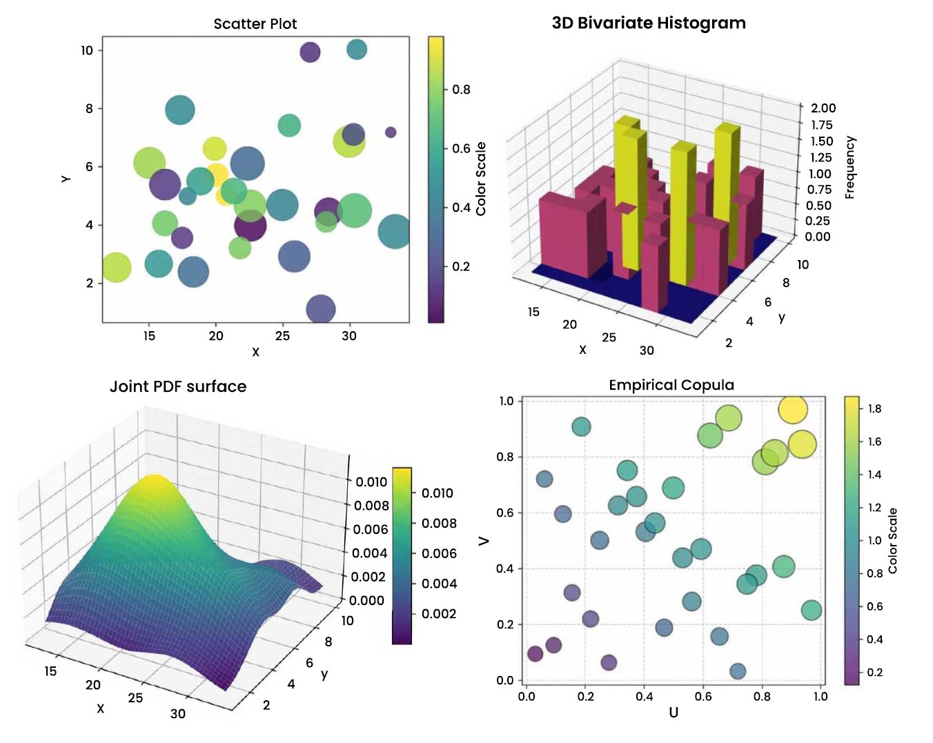
The first dataset is the economic dataset presented in Table 6. It contains 31 annual time-series observations from 1980 to 2010, consisting of the response variables: exports of goods and services  and GDP growth [30].
Table 6. Observations of the first and second dataset.
| Economic Dataset | Environmental Dataset | |||||||
| Years | X | Y | No. | X | Y | No. | X | Y |
| 1980 | 30.51 | 10.01 | 1 | 99 | 12 | 32 | 90 | 7 |
| 1981 | 33.37 | 3.76 | 2 | 61 | 17 | 33 | 22 | 20 |
| 1982 | 27.03 | 9.91 | 3 | 86 | 7 | 34 | 72 | 4 |
| 1983 | 25.48 | 7.4 | 4 | 113 | 13 | 35 | 176 | 7 |
| 1984 | 22.35 | 6.09 | 5 | 96 | 5 | 36 | 107 | 6 |
| 1985 | 19.91 | 6.6 | 6 | 99 | 2 | 37 | 84 | 12 |
| 1986 | 15.73 | 2.65 | 7 | 83 | 12 | 38 | 83 | 10 |
| 1987 | 18.84 | 2.52 | 8 | 57 | 2 | 39 | 37 | 20 |
| 1988 | 17.32 | 7.93 | 9 | 80 | 6 | 40 | 67 | 3 |
| 1989 | 17.89 | 4.97 | 10 | 79 | 4 | 41 | 83 | 12 |
| 1990 | 20.05 | 5.7 | 11 | 75 | 5 | 42 | 36 | 3 |
| 1991 | 27.82 | 1.08 | 12 | 70 | 14 | 43 | 49 | 18 |
| 1992 | 28.4 | 4.43 | 13 | 15 | 6 | 44 | 39 | 18 |
| 1993 | 25.84 | 2.9 | 14 | 62 | 2 | 45 | 102 | 14 |
| 1994 | 22.57 | 3.97 | 15 | 87 | 4 | 46 | 66 | 14 |
| 1995 | 22.55 | 4.64 | 16 | 95 | 18 | 47 | 154 | 8 |
| 1996 | 20.75 | 4.99 | 17 | 81 | 4 | 48 | 72 | 6 |
| 1997 | 12.56 | 5.49 | 18 | 71 | 19 | 49 | 63 | 22 |
| 1998 | 16.21 | 4.04 | 19 | 44 | 5 | 50 | 83 | 11 |
| 1999 | 15.05 | 6.11 | 20 | 13 | 14 | 51 | 77 | 8 |
| 2000 | 16.2 | 5.37 | 21 | 52 | 40 | – | – | – |
| 2001 | 21.35 | 3.54 | 22 | 97 | 8 | – | – | – |
| 2002 | 18.32 | 2.37 | 23 | 146 | 11 | – | – | – |
| 2003 | 21.8 | 3.19 | 24 | 52 | 26 | – | – | – |
| 2004 | 28.23 | 4.09 | 25 | 52 | 1 | – | – | – |
| 2005 | 30.34 | 4.48 | 26 | 29 | 3 | – | – | – |
| 2006 | 29.95 | 6.85 | 27 | 108 | 10 | – | – | – |
| 2007 | 30.25 | 7.09 | 28 | 135 | 18 | – | – | – |
| 2008 | 33.04 | 7.16 | 29 | 102 | 6 | – | – | – |
| 2009 | 24.96 | 4.67 | 30 | 48 | 10 | – | – | – |
| 2010 | 17.48 | 5.15 | 31 | 66 | 23 | – | – | – |
7.2. Modelling Environmental Data
The second dataset is the environmental dataset presented in Table 6. The dataset contains observations from 51 major cities in the United States, where represents the average precipitation (in millimeters) and  represents the average maximum temperature (in degrees Celsius). This data was compiled by the National Climatic Data Center (NCDC), USA, and are publicly accessible via their official website https://www.ncei.noaa.gov/.
The fit of FGM Bivariate Generalized Inverse Weibull Distribution (FGM GIW) is compared with a number of alternative probability distributions under FGM family such as FGM Lomax Distribution (FGM LD), FGM Inverse Lomax Distribution (FGM ILD), FGM Weibull Distribution (FGM WD), FGM Inverse Weibull Distribution (FGM IWD) and FGM Burr XII Distribution (FGM BXD). Several criteria are utilized to evaluate the performance of these models such as Akaike Information Criteria (AIC), Bayesian Information Criteria (BIC), Corrected Akaike Information Criteria (CAIC) and Hannan Quinn Information Criteria (HQIC).
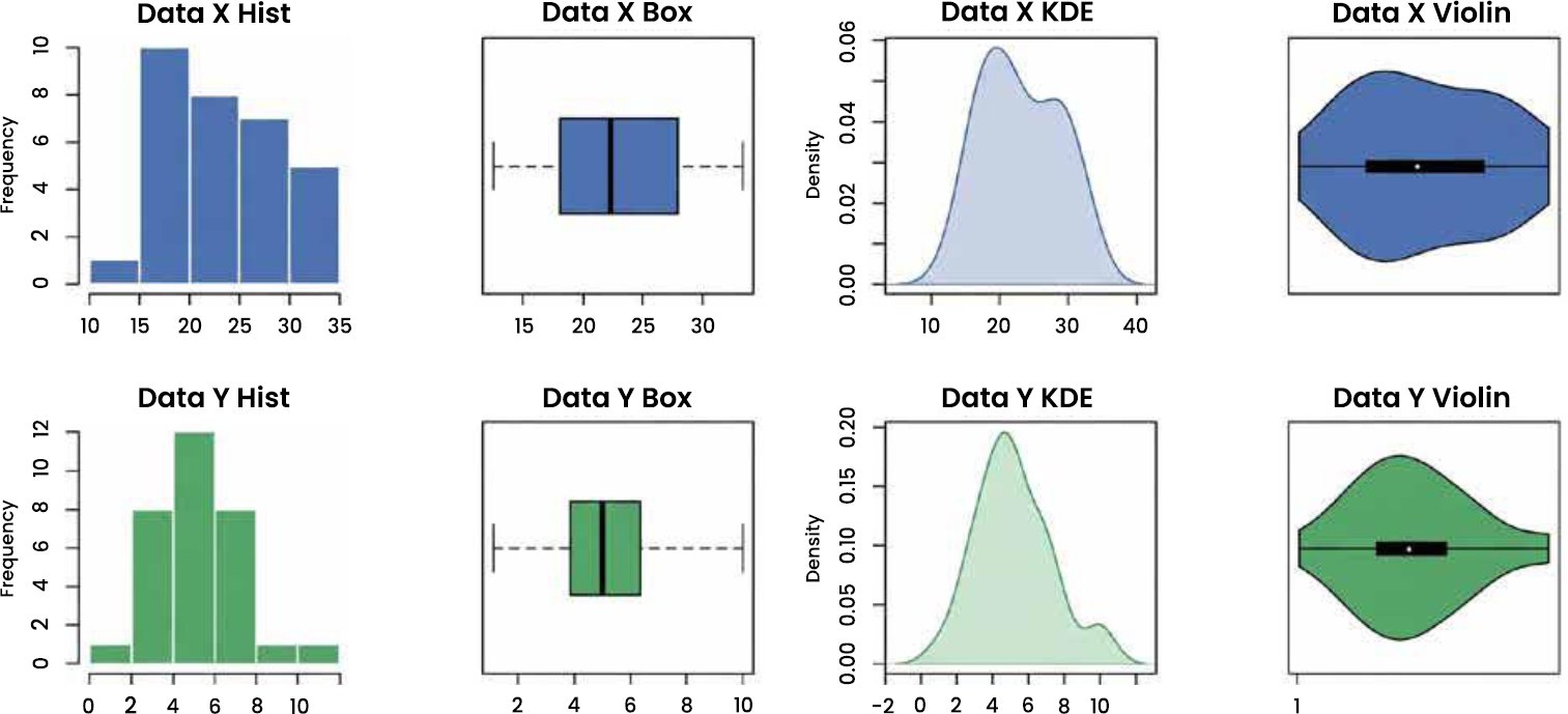
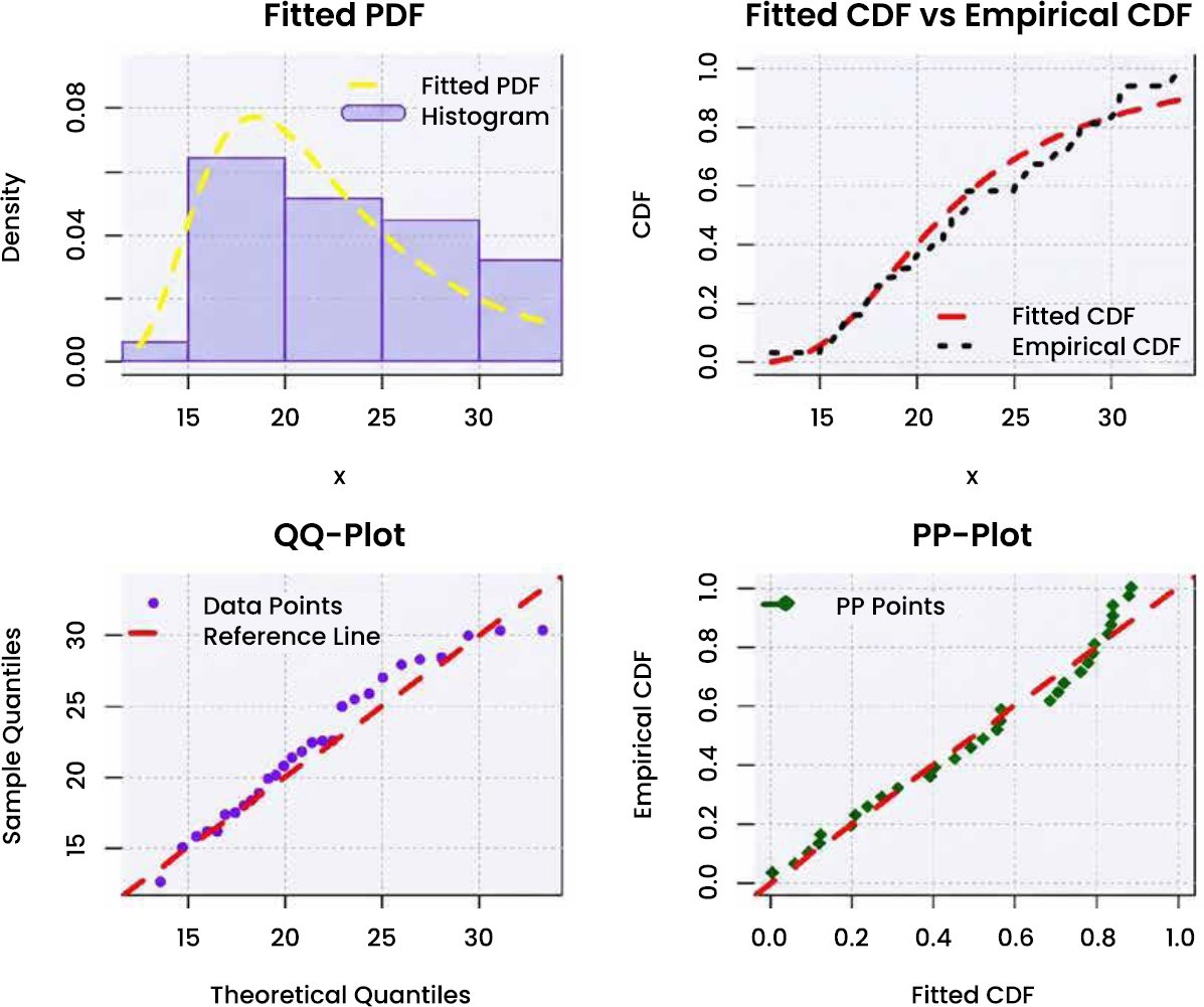
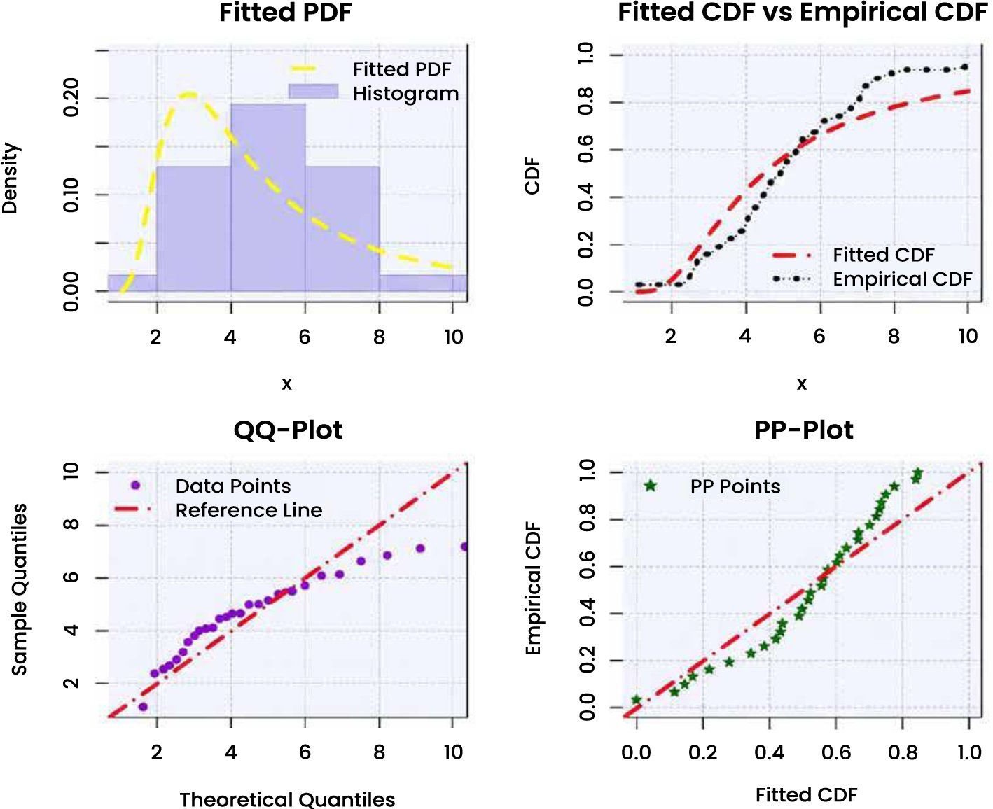
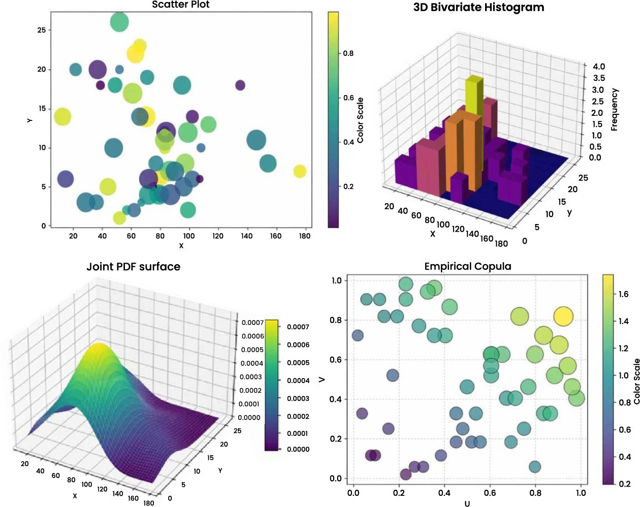
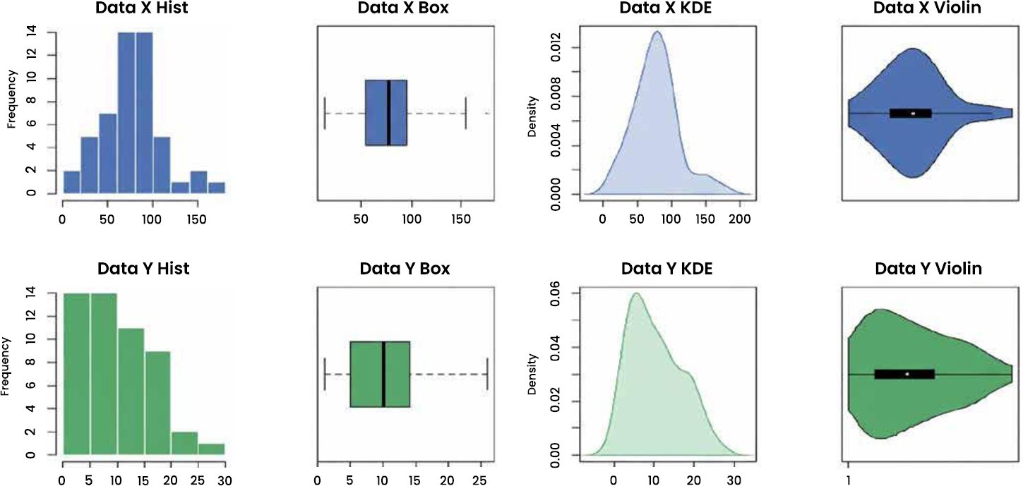
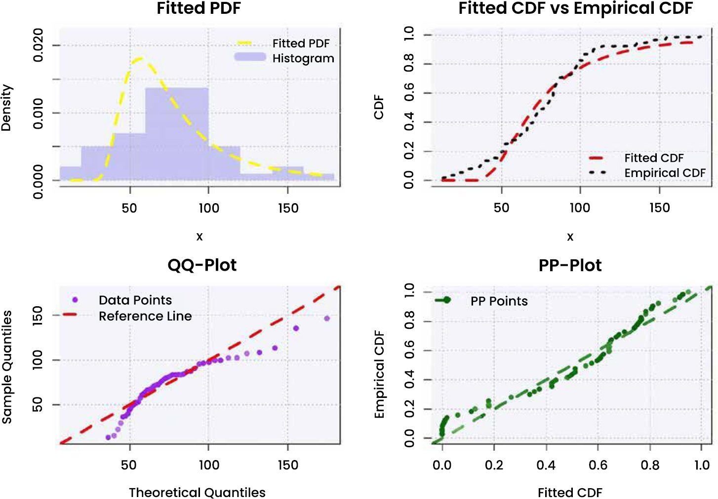
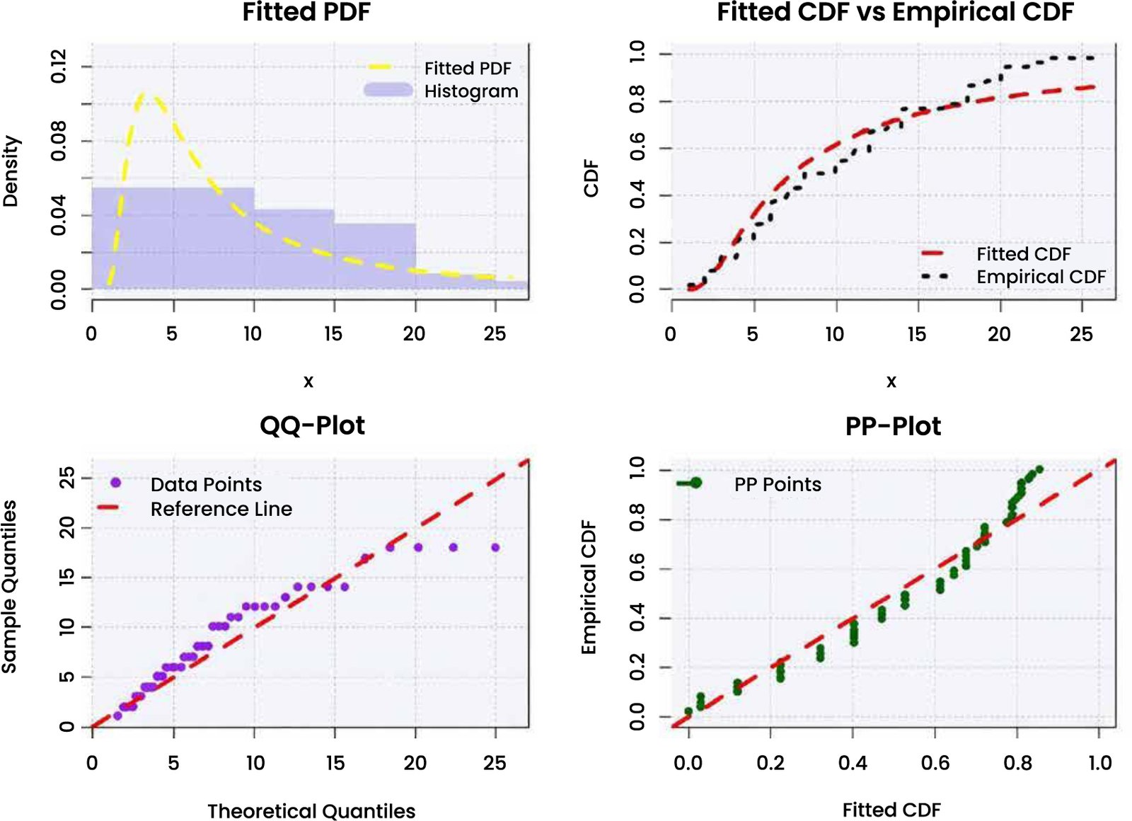
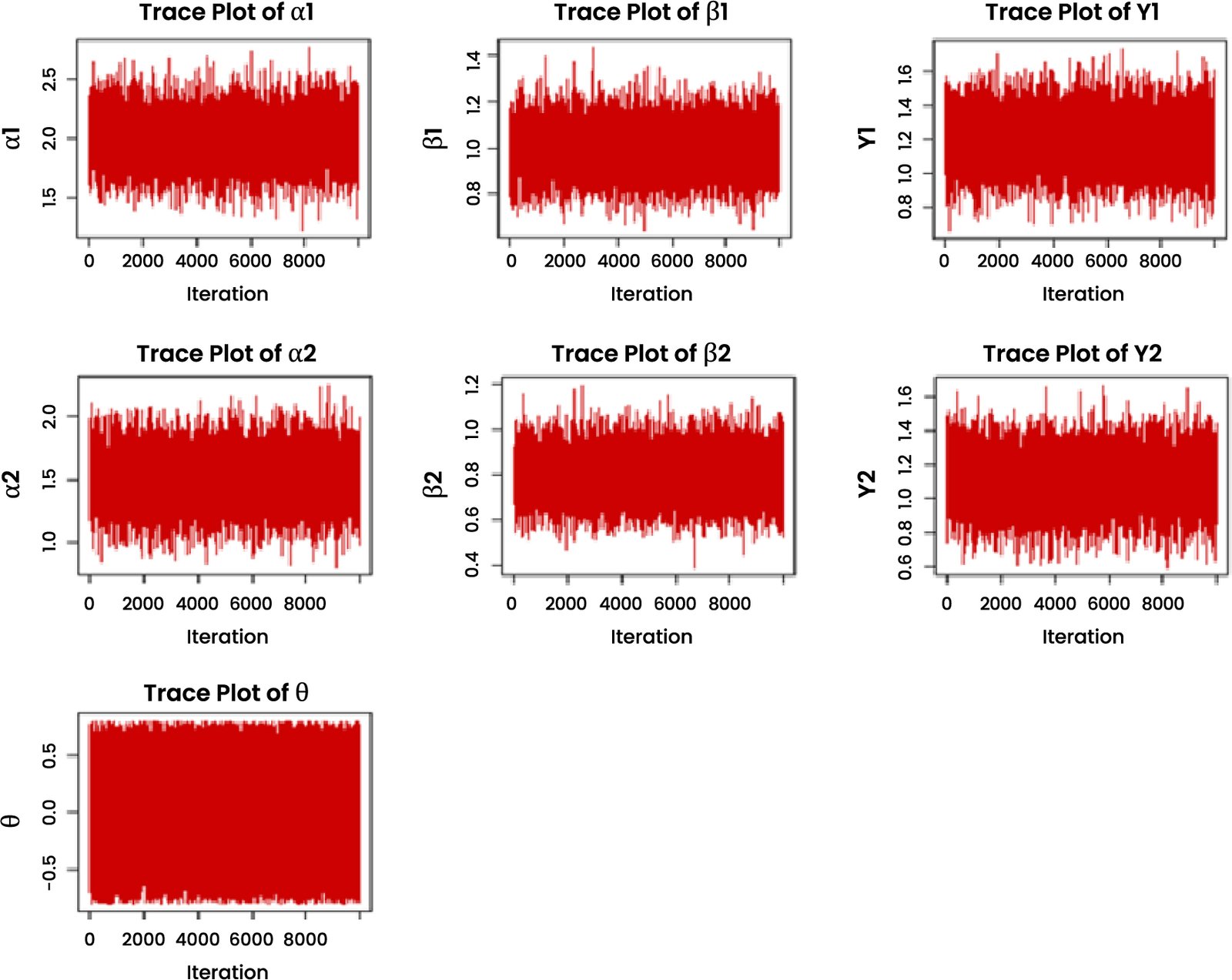
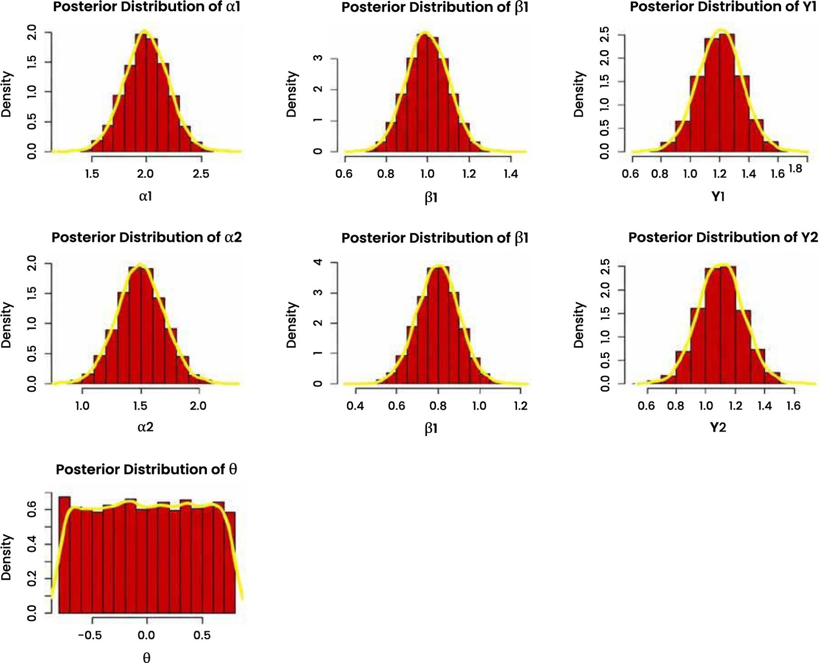
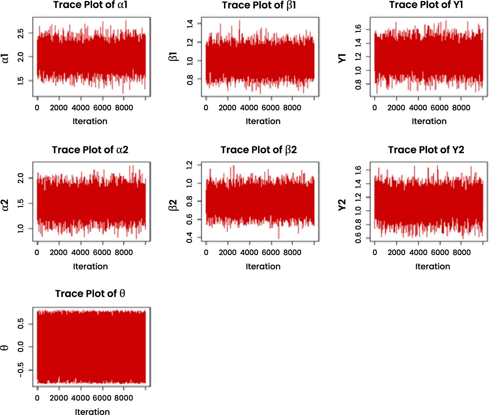
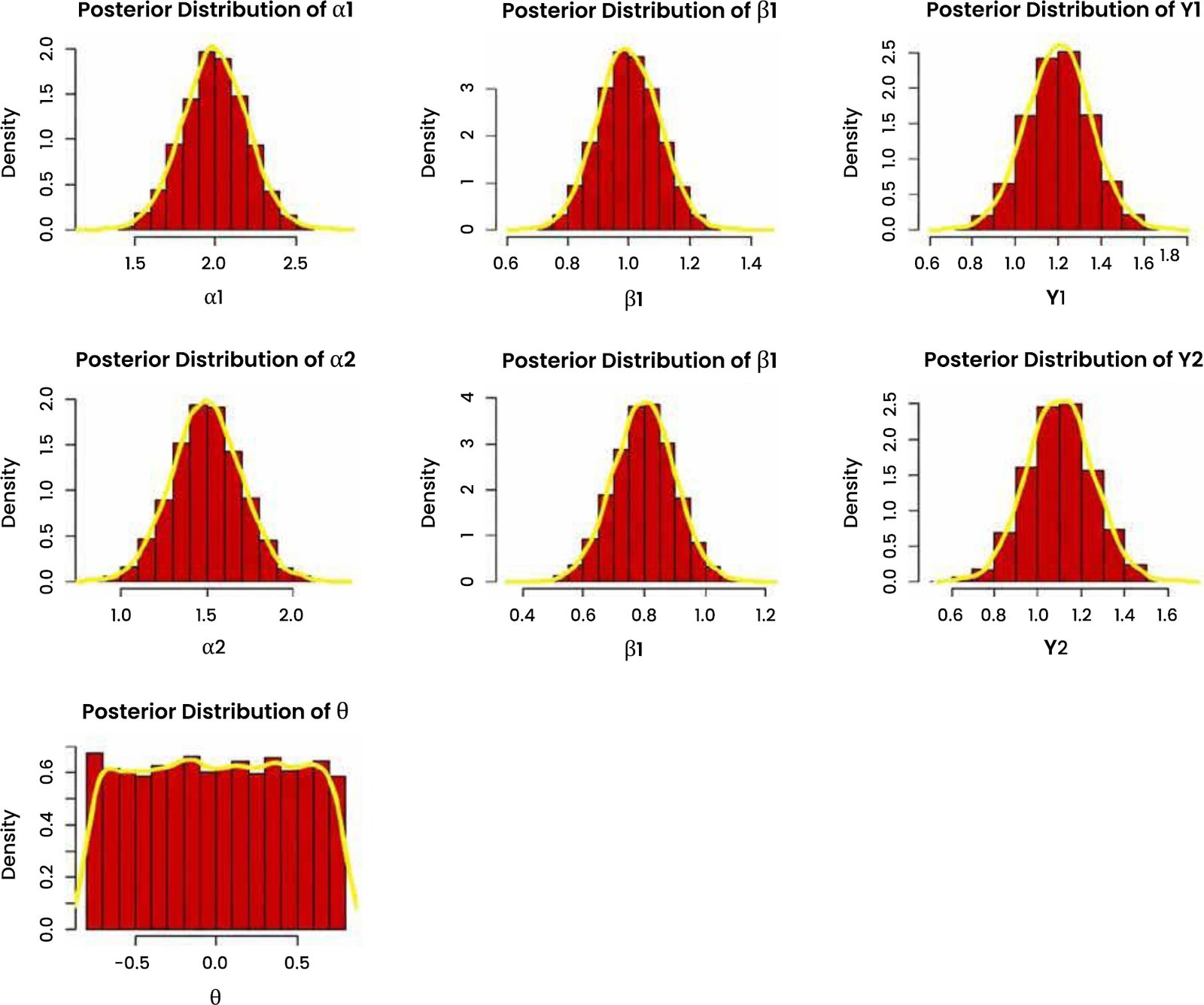
The goodness of fit results presented in Tables 9 and 12 indicates that the FGM-GIW distribution provides the best fit among the considered models, consistently yielding the lowest values across all information criteria. This demonstrates the flexibility and capability of the proposed FGM-GIW distribution in modeling the two datasets. Furthermore, Tables 7 and 10 presents the parameter estimates, while Tables 8 and 11 shows the maximum likelihood and Bayesian estimates for the marginal distributions. To illustrate the datasets, a basic statistical analysis including scatter plot, bivariate histogram, joint PDF surface plot and empirical copula is provided in Figs. (6 and 10). Univariate graphical representation including histogram, boxplot, kernel density and violin plot of both datasets are shown in Figs. (7 and 11). The fitted plots, including fitted PDFs, fitted CDFs, QQ-plots, and PP-plots of the marginal distributions, are presented in Figs. (8, 9, 12, and 13). Finally, the MCMC results are displayed in Figs. (14, 15, 16 and 17).
Table 7. Parameter estimates of FGM-GIW for the economic data.
| Parameters | MLE | IFM | Bayesian |
| | 10.00 | 10.00 | 12.4611 |
| | 3.5420 | 3.5220 | 3.51805 |
| | 10.00 | 10.000 | 4.88734 |
| | 2.2669 | 2.0738 | 2.58490 |
| | 1.8026 | 1.7853 | 1.75637 |
| | 2.3492 | 2.7680 | 2.28862 |
| | 0.8718 | 0.8763 | 0.31457 |
Table 8. MLE and Bayesian estimates for the marginal distributions for the economic data.
| – | Parameters | MLE | Bayesian |
| | | 11.1957 | 12.49365 |
| | 3.99212 | 3.367972 | |
| | 9.24951 | 4.554247 | |
| | | 4.21177 | 3.06655 |
| | 1.78539 | 1.732717 | |
| | 0.78133 | 2.056865 |
Table 9. Goodness of fit for economic data.
| Models | Log-likelihood | AIC | BIC | CAIC | HQIC |
| FGM-GIW | -174.6655 | 363.331 | 373.369 | 380.369 | 366.6032 |
| FGM-LD | -181.3567 | 374.713 | 384.7504 | 391.7504 | 377.9854 |
| FGM-ILD | -183.9082 | 379.816 | 389.8534 | 396.8534 | 383.0884 |
| FGM-WD | -186.4425 | 384.885 | 394.9220 | 401.9220 | 388.1570 |
| FGM-IWD | -189.0173 | 390.034 | 400.0716 | 407.0716 | 393.3066 |
| FGM-BXD | -192.5531 | 397.106 | 407.1432 | 414.1432 | 400.3782 |
Table 10. Parameter estimates of FGM-GIW for the environmental data.
| Parameters | MLE | IFM | Bayesian |
| | 10.1001 | 10.0200 | 11.61156 |
| | 1.4323 | 1.4318 | 1.3652 |
| | 10.2235 | 10.2150 | 8.3365 |
| | 2.2268 | 2.56240 | 2.7877 |
| | 1.2230 | 1.2217 | 1.2153 |
| | 3.0397 | 2.5650 | 2.7287 |
| | 0.0473 | 0.04308 | 0.00738 |
Table 11. MLE and Bayesian estimates for the marginal distributions for the environmental data.
| – | Parameters | MLE | Bayesian |
| | | 12.1441 | 9.9855 |
| | 1.5421 | 1.3251 | |
| | 9.3311 | 8.6927 | |
| | | 4.5500 | 2.9234 |
| | 1.2217 | 1.2017 | |
| | 1.2717 | 2.5605 |
Table 12. Goodness of fit for environmental data.
| Models | Log-likelihood | AIC | BIC | CAIC | HQIC |
| FGM-GIW | -440.1218 | 894.243 | 907.7663 | 914.7663 | 899.411 |
| FGM-LD | -447.9124 | 907.824 | 921.3481 | 928.3481 | 912.9928 |
| FGM-ILD | -450.3067 | 912.613 | 926.1367 | 933.1367 | 917.7814 |
| FGM-WD | -453.8895 | 919.779 | 933.3023 | 940.3023 | 924.9470 |
| FGM-IWD | -457.2148 | 926.429 | 939.9529 | 946.9529 | 931.5976 |
| FGM-BXD | -461.8803 | 935.760 | 949.2839 | 956.2839 | 940.9286 |