

pdpublishers.com

Journal-of-Information-Technology-and-Scientific-Innovation
Table of Contents

Article ID: PD2601202007

Views: 545
Volume 1 (2026)
Published 06 Oct 2026

Leakage-Aware Robotic Grasping: Experiment-Level Explainable Robustness Prediction and Retrospective Effort-Aware Assessment

📚 Cited by: 0

⬇ Downloads: 30


Author

1Faculty of Computer Science & Information Technology, University Putra Malaysia, Selangor, Malaysia

Article History:

Received: 16 June, 2026

Accepted: 15 September, 2026

Revised: 08 September, 2026

Published: 06 October, 2026

ABSTRACT:

Introduction: Robotic grasping produces repeated proprioceptive measurements whose experimental hierarchy can make flat-table evaluation overly optimistic.

Methodology: The paper analyses the Shadow Robot Smart Grasping Sandbox benchmark, comprising 992,641 measurement rows nested within 53,937 simulated grasp experiments with one released robustness target per experiment. The novelty is methodological rather than architectural: compared with prior work on this benchmark centred on grasp classification, failure prediction, or local explainability, we formulate experiment-level robustness regression and combine experiment-disjoint splitting, inverse experiment-size weighting, fold-local preprocessing, identifier-free attribution, robustness diagnostics, and effort-aware assessment in one reproducible pipeline.

Results: On 10,788 unseen holdout experiments, R² was 0.5386 for Linear Regression, 0.6539 for MLP, 0.7104 for XGBoost, and 0.7132 for the stacked ensemble; XGBoost achieved MAE = 9.52, median absolute error = 5.11, and Spearman ρ = 0.915. Five-fold target-decile-stratified validation gave pooled out-of-fold R² = 0.8687, while a single out-of-range holdout target accounted for most squared error.

Conclusion: Paired bootstrapping indicated no material practical advantage from stacking. The results are limited to completed simulated episodes, with physical transfer and prospective online operation left for future validation.

Keywords: Robotic grasping, grasp robustness, proprioception, group-aware validation, experiment-level evaluation, explainable AI, XGBoost, ensemble learning, retrospective effort-aware assessment.

1. INTRODUCTION

Robotic grasping is central to manipulation in manufacturing, logistics, healthcare and assistive systems [1]. Compliant and soft grippers are particularly attractive because mechanical adaptation can improve contact with uncertain or fragile objects, but compliance also makes modelling and control more difficult [2]. The benchmark analysed in the present study, however, is the Shadow Robot Smart Grasping Sandbox simulation of a robotic hand; it does not provide measurements of material stiffness, strain, deformation fields, elastomer behaviour, pneumatic pressure, tendon compliance, material composition or constitutive parameters. Soft-robotics and material-intelligence research are therefore used as broader motivation and comparison, not as a direct description of the measured dataset.

Robotic grasping research spans explicit physical models, kinematics and contact assumptions as well as increasingly data-driven approaches [3]. Analytical methods can become difficult when contact conditions are uncertain or the state space is high-dimensional. A complementary data-driven strategy learns relationships between measured robot states and grasp outcomes [4]. The current benchmark focuses on recorded joint position, velocity and effort channels rather than observed soft-body deformation.

Machine-learning techniques can model nonlinear input-output relationships in robotic manipulation without requiring an analytical representation of every contact interaction. Proprioceptive, tactile, visual and actuator signals have been employed for grasp assessment and control in previous studies [5]. This motivates the present emphasis on structured joint-state measurements and the careful separation of physical variables from data identifiers.

A major challenge in data-driven grasp modelling is generalisation beyond the training data. When multiple measurements are recorded within the same grasp experiment, states from that experiment are not statistically interchangeable with measurements from independent experiments. Complete experiments, rather than individual rows, must therefore be separated between training and evaluation sets.

Artificial-intelligence methods can learn task-relevant representations from sensory data and can complement model-based grasping approaches. Supervised models estimate outcomes from observed robot states, whereas reinforcement learning improves policies through interaction [6]. The present study uses supervised robustness regression and a supervisory decision-support formulation rather than an autonomous control policy.

Robotic grasping datasets have diverse sensing modalities and experimental designs. The Cornell Grasping Dataset is a standard vision-based grasp dataset with annotated grasp rectangles [7], while the Shadow Smart Grasping benchmark analysed in this work is a simulated dataset of repeated measurements of grasping joint states in grasp experiments [8]. This structure is convenient for modelling proprioceptive tasks, but it poses a particular leakage problem when rows of measurements from one experiment are split between the training and test sets. In this study, we therefore differentiated experiment-level units from within-experiment measurements throughout the methodology.

Existing Smart Grasping studies have mainly addressed grasp classification, failure prediction, or explainability, while broader robot-learning studies emphasise visual grasp detection or multimodal action-generation policies [9, 10]. Those tasks do not answer whether a continuous robustness score generalises across complete, previously unseen grasp experiments when repeated measurement rows, unequal episode lengths, and identifier fields are present. This experiment-structure problem, rather than a search for a new model architecture, motivates the present study.

This study therefore treats robustness estimation as experiment-level supervised regression. It develops a leakage-controlled framework that compares linear, tree-based, neural and stacked regressors under experiment-disjoint validation; equalises each experiment’s training influence; fits preprocessing only on legally available training groups; removes identifiers before explanation; quantifies extreme-case, bootstrap, ablation and synthetic-noise robustness; and includes a post-episode effort–robustness assessment. The analysis is scoped to completed simulated episodes.

2. LITERATURE REVIEW

2.1. Robotic Grasping, Compliance and Material-Aware Context

Conventional rigid manipulation can be extended to soft robots, which rely on compliant materials such as elastomers, smart polymers and hydrogels [11, 12]. These materials can deform and recover after large deformations, enabling soft devices to flex, extend and conform to objects with complex geometry. Soft systems incorporate flexible structures and may operate with less precise kinematic control than rigid manipulators. This literature provides broader context for compliant manipulation; the Shadow Smart Grasping benchmark itself does not contain direct material-property or soft-body-deformation measurements.

The mechanical behaviour of different classes of soft materials varies and is relevant to compliant robotic manipulation. Shape-memory polymers can change their shape when exposed to heat or electricity, and hydrogels can expand or shrink when the temperature or pH changes. Many other materials are used to manufacture compliant grippers, including elastomers like silicone and polyurethane, which can withstand repeated deformations [13, 14]. These material characteristics encourage studies of compliant grasping, but are not features in the data assessed here.

Compliance can make physical adaptation easier and modelling and control more difficult. By incorporating passive deformation, a gripper can conform to different object shapes without precisely controlling its position at each point of contact. Meanwhile, deformation may be history-dependent and nonlinear, and it is very sensitive to contact conditions, making analytical models difficult to develop [15–17]. The challenges stimulate data-driven grasp analysis but, in the present benchmark, only joint-state and effort measurements, not deformations, are provided.

2.2. AI in Robotics

Artificial intelligence is increasingly used to model complex mappings between robot states, sensory inputs and task outcomes. Grasp-related classification and prediction have employed decision trees, random forests and support-vector machines [18]. These methods can accommodate nonlinear or high-dimensional data without assuming a specific soft-robot platform.

Large data sets can be used to learn hierarchical representations using deep learning techniques. CNNs have performed relatively well on vision-based grasp detection, while recurrent neural networks and long short-term memory models are good for sequential sensorimotor signals such as actuator and proprioceptive time series [19]. Relations between joints or sensing elements can also be used to represent the structure of the robots by graph neural networks. An argument that the data on this flat table is intrinsically sequential is not made, these model families are discussed as methodological background, not as evidence of that.

High-capacity learning models can be difficult to interpret, which is important in physically interactive systems. Explainability can help identify which recorded variables contribute to model outputs and can expose reliance on nonphysical fields such as identifiers [20]. In this benchmark, experiment_number and measurement_number describe data organisation rather than robotic sensing.

Reinforcement learning (RL) interacts with an environment to learn manipulation and grasping policies [21, 22]. RL is not used in this study; it is discussed only as a potential extension. More generally, simulation-to-real transfer remains challenging because simulated contact and sensing may not reproduce all sources of physical uncertainty [23].

Recent foundation-robotics research has shifted from task-specific predictors toward generalist vision-language-action (VLA) policies. RT-2 demonstrated that robot actions can be represented as tokens within a VLA model and evaluated the resulting policy over thousands of trials [24]. Octo subsequently introduced an open-source generalist policy trained on approximately 800,000 robot trajectories across multiple embodiments [25], while OpenVLA scaled this direction to a 7-billion-parameter model trained on 970,000 real-world demonstrations and reported improved task-success generalisation relative to RT-2-X and Diffusion Policy baselines [26]. In parallel, 3D Diffusion Policy (DP3) combined sparse 3D representations with diffusion-based action generation, reporting a 24.2% relative improvement over baselines across 72 simulated tasks and 85% success on four real-robot tasks [27]. The π₀ model further extended foundation robotics through a vision-language-action flow-matching policy trained across diverse robot platforms and dexterous manipulation tasks [28]. Recent reviews identify multimodal grounding, cross-embodiment generalisation, uncertainty, safety, and real-time deployment as continuing challenges for foundation models and VLAs in robotics [29, 30].

These generalist developments provide important context but solve a different learning problem from the present work: they generate actions from multimodal observations and instructions, whereas the current study estimates a scalar robustness score from internal sensor states only. At the hardware level, recent soft and tactile robotic hands have also advanced dense contact sensing and compliant manipulation; for example, TacPalm SoftHand coordinates tactile palm sensing with soft fingers [31], while a 2026 tactile-reactive gripper integrates an active tactile palm with compliant fingers for dexterous manipulation [32]. These studies reinforce the value of physically meaningful sensing, while the present benchmark deliberately isolates proprioceptive joint-position, joint-velocity, and joint-effort information.

A recurring issue in high-performing models is that feature attribution can be confused with physical explanation. Explainable-AI studies of industrial robots show the value of tracing model outputs to joint-level variables [33]. The present work therefore separates physical joint channels from dataset identifiers, because identifier importance can reveal data-structure leakage rather than dependence on meaningful robot-state variables.

2.3. Datasets in Robotic Grasping

Benchmark datasets have strongly influenced learning-based robotic grasping. The Cornell Grasping Dataset provides RGB-D images with annotated grasp rectangles and is primarily a vision-based grasp-detection benchmark [7]. It does not provide the repeated proprioceptive experiment structure that characterises the Shadow Smart Grasping benchmark used in the present study.

Other grasping datasets extend visual grasp detection to larger object and annotation collections; large-scale grasp-detection resources are surveyed in [34, 35], while the Jacquard dataset provides a large collection of synthetic grasp annotations [36]. Such resources address different tasks and sensing assumptions from the present proprioceptive regression problem, so their performance metrics are not directly interchangeable.

BC-Z addresses zero-shot task generalisation with robotic imitation learning using vision-based observations and task conditioning rather than continuous grasp-robustness regression [37]. This illustrates the diversity of modern manipulation datasets and objectives. The Shadow Smart Grasping benchmark considered here instead provides repeated measurements of joint position, velocity and effort during simulated grasp experiments; its experiment/measurement hierarchy must therefore be preserved during validation [8, 9].

2.4. Research Gap & Novelty

The novelty of this work is methodological rather than architectural. The contribution is a defensible experiment-level evaluation for a repeated-measurement grasp benchmark: complete grasp experiments, not rows, define the independent unit; unequal episode lengths are balanced during training; preprocessing is fold-local; identifiers are excluded from the model and explanation spaces; and robustness, uncertainty and effort trade-offs are evaluated at the experiment level.

This scope is intentionally narrower than material-aware or closed-loop robotic control. The benchmark contains joint configuration, instantaneous joint motion and actuator effort/torque-equivalent signals, but no direct measurements of stiffness, strain, deformation, pneumatic pressure, material composition, electrical energy or real-robot sensing. Accordingly, material-mechanism and sensor-validation claims are outside the evidential scope of the dataset.

Relative to the closest Shadow Smart Grasping studies, Sabeeh [9] evaluates grasp-stability classification, whereas Alvanpour et al. [38] and Acun et al. [39] focus on grasp-failure prediction and explainability. The present work instead targets a continuous released robustness score and asks whether that score can be predicted for experiment-disjoint grasps under group balancing, leakage-controlled preprocessing, identifier-free attribution and explicit extreme-case reliability analysis. These differences define the substantive novelty shown in Table 1.

Table 1. Comparison with recent published robotic learning and grasping methods.

StudySetting / InputMethod / ObjectiveReported Performance and Relation to Present Study
Sabeeh (2024) [9]Smart Grasping Sandbox; joint position, velocity, effortDNN/CNN/LSTM grasp-stability classification≈96% test accuracy for the proposed DNN; CNN 94.12%; LSTM 91.81%. Same benchmark family, but classification rather than continuous regression.
Kim et al. (2025), OpenVLA [26]970k real-world robot demonstrations; vision + language + action7B generalist VLA policyReported +16.5 percentage-point task-success improvement over RT-2-X across 29 tasks and +20.4 points over Diffusion Policy after task-specific fine-tuning; different multimodal control task.
Ze et al. (2024), DP3 [27]72 simulated tasks + 4 real-robot tasks; sparse 3D observations3D diffusion visuomotor policy24.2% relative improvement over baselines in simulation; 85% success on four real-robot tasks. Action-generation objective, not scalar robustness regression.
Acun et al. (2025) [39]Shadow Smart Grasping; simulated joint statesBlack-box grasp-failure predictor with local explainabilityPredictor AUC = 0.8340. Same benchmark family, but binary failure prediction and explanation fidelity rather than continuous R².
Zhang et al. (2025) [31]; Zhou et al. (2026) [32]Physical soft/tactile robotic handsTactile palm–finger coordination and tactile-reactive dexterous manipulationPhysical-system demonstrations emphasise tactile sensing, compliance, and dexterity; no directly comparable continuous robustness R² is reported.
Present study992,641 measurement rows nested within 53,937 experiments; 27 physical position/velocity/effort variablesExperiment-level regression + group balancing + reproducible stacking + identifier-free XAI + retrospective effort–robustness Pareto assessmentExperiment-disjoint holdout: XGBoost R² = 0.7104; stacked ensemble R² = 0.7132. Five-fold XGBoost pooled out-of-fold R² = 0.8687. Metrics are computed over unique experiments.

Accordingly, the study contributes a single reproducible pipeline linking continuous experiment-level regression, equalised experiment influence, target-stratified stability analysis, paired bootstrap model comparison, identifier-free explanation, synthetic perturbation stress testing and post-episode Pareto assessment. Generalist policies such as Octo, OpenVLA, DP3 and π₀ [25–28] remain important contextual comparators, but they address multimodal action generation rather than this experiment-level scalar estimation problem.

Table 1 provides contextual comparison with recent robotic learning and grasping studies. The cited studies use different datasets, targets, sensing modalities, robot platforms and metrics, so their numerical values are contextual rather than head-to-head benchmarks. The present study now reports confirmatory experiment-level results generated under experiment-disjoint validation; archived row-level values are no longer used as the principal evidence.

3. METHODOLOGY

3.1. Executed Leakage-Controlled Pipeline

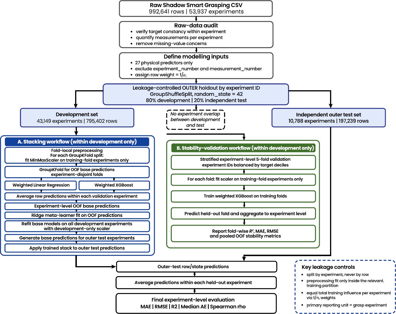
Fig. (1) distinguishes three purposes that were previously easy to conflate. The outer experiment-disjoint holdout provides the primary generalisation estimate. Stacking uses five-fold GroupKFold only within the outer development partition, with a fresh MinMaxScaler fitted inside every base-training fold before out-of-fold prediction. Separately, the five-fold stability analysis stratifies all 53,937 experiment IDs by target decile and fits a fresh scaler inside every training fold. Final state-conditioned estimates are aggregated across the complete recorded episode.

Fig. (1). Leakage-controlled outer holdout, stacking and stability-validation workflow.

3.2. Dataset Description

This study utilised the publicly available Grasping Dataset generated in the Shadow Robot Smart Grasping Sandbox simulation environment. Direct analysis of the supplied raw CSV confirmed 992,641 measurement rows organised into 53,937 simulated grasp experiments. Experiments contain between 1 and 30 recorded measurement states (mean 18.40, median 15, interquartile range 13–30). No missing numerical values were detected. During an experiment, the robotic hand grasps a ball and undergoes a shaking procedure while joint states are recorded.

The simulated Shadow hand has three fingers with three articulated joints per finger. Each of the nine joints contributes three physical channels: position, velocity and effort/torque-equivalent feedback. The physical proprioceptive input space therefore contains 9 × 3 = 27 variables: nine position variables, nine velocity variables and nine effort variables. The remaining non-target fields include experiment_number and measurement_number, which identify the experiment and the within-experiment measurement order; they are metadata and are excluded from the leakage-controlled predictor matrix.

The data hierarchy is defined as follows. Level 1 – experiment/grasp: one simulated grasp-and-shake episode and the independent unit for generalisation (53,937 experiments). Level 2 – measurement/state: a repeated joint-state recording within an experiment (1–30 rows). Level 3 – dataset row: one state containing experiment and measurement identifiers, 27 physical joint variables and the experiment-level robustness target. The raw-data audit verified that robustness has exactly one unique value within every experiment (53,937/53,937 groups), so the same outcome is repeated across that experiment’s measurement rows.

The scientific task is supervised continuous regression: use internal proprioceptive states from a previously unseen grasp experiment to estimate that experiment’s released robustness target. Because all states in one experiment share the same target, complete experiments are the independent units for splitting and evaluation. Models produce state-conditioned estimates, but confirmatory performance is calculated only after averaging all states from the completed held-out episode. Accordingly, the validated task is retrospective full-episode estimation rather than causal inference, early-warning prediction or autonomous control.

3.2.1. Joint Positions (pos):

Position channels record simulated joint-angle/encoder readings (radians) for the articulated degrees of freedom of the Shadow hand. They describe the geometric arrangement of the fingers at each measurement state and therefore encode enclosure, fingertip alignment, and grasp configuration.

3.2.2. Joint Velocities (vel):

Velocity channels represent the temporal rate of change of joint position reported by the simulator. They characterise instantaneous motion during grasp execution or adjustment, including transient corrective movements and fine positioning around contact.

3.2.3. Joint Efforts (eff):

Effort channels correspond to simulated actuator torque feedback for the joints. They provide a torque-equivalent measure of actuator loading and therefore serve as a proxy for internal force generation during contact and grasp maintenance; they are not direct measurements of electrical energy consumption.

The retrospective assessment compares predicted experiment-level robustness against the observed mean-absolute effort descriptor Cᵢ. Direct raw-data verification found one and only one robustness value within every experiment; that value is repeated unchanged across all of the experiment’s measurement rows. Let xᵢⱼ denote the 27-dimensional physical proprioceptive vector measured at state j in experiment i, and let Rᵢ denote the single released robustness target for experiment i. The model learns xᵢⱼ → Rᵢ at the state level, while generalisation is evaluated after aggregating predictions to one R̂ᵢ per unseen experiment.

3.2.4. Benchmark Target Definition

Published descriptions of the Smart Grasping benchmark relate robustness to the stability or variation of the palm-to-ball distance during the shake experiment [8, 9, 39]. The raw dataset confirms the target’s experiment-level repetition but does not provide the provider’s closed-form scoring transformation. Equation (1) is therefore schematic rather than a reconstructed scoring law.

      (1)

where Δdₚₐₗₘ–ᵦₐₗₗ(eᵢ) denotes palm-to-ball distance variation for experiment eᵢ and f (·) denotes the dataset provider’s scoring transformation. The present study predicts the released target directly and does not claim to reconstruct or recalibrate f (·).

   (2)

where G is the number of development experiments and nᵢ is the number of measurement states in experiment i. Implementationally, each measurement row receives sample weight 1/nᵢ, normalised to mean weight 1 for numerical convenience. Thus every grasp experiment contributes equal total weight to the training loss despite unequal numbers of recorded states.

To estimate generalisation to unseen grasps, GroupShuffleSplit created an 80/20 experiment-disjoint holdout from the experiment identifiers with random seed 42 before any scaler was fitted. The development partition contained 43,149 experiments (795,402 rows) and the test partition 10,788 experiments (197,239 rows), with zero experiment overlap. This outer split was not stratified by target and was never used for hyperparameter selection. Model construction and stacking were confined to development experiments.

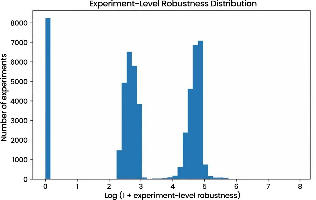
Higher released target values represent higher benchmark grasp-quality scores. Because robustness is constant within each experiment, descriptive and inferential summaries are reported at experiment level. Across the 53,937 unique experiments, robustness had mean 53.03, SD 53.93, median 16.72, interquartile range 11.61–106.04, minimum 0.000001 and maximum 2933.58; skewness was 3.385, confirming a strong upper tail.

Row-weighted descriptive statistics are no longer used to characterise the independent sample because experiments have unequal row counts. A 30-state grasp would otherwise contribute six times as many rows as a 5-state grasp. Table 2 therefore reports the audited hierarchy, measurement-count distribution and experiment-level target statistics.

Table 2. Dataset hierarchy and experiment-level descriptive statistics.

StatisticValue
Measurement rows992,641
Independent experiments53,937
Measurements/experiment: minimum1
Measurements/experiment: 25th percentile13
Measurements/experiment: median15
Measurements/experiment: mean18.40
Measurements/experiment: 75th percentile30
Measurements/experiment: maximum30
Experiments with constant robustness53,937 / 53,937 (100%)
Experiment-level robustness mean53.03
Experiment-level robustness SD53.93
Experiment-level robustness minimum0.000001
Experiment-level robustness 25th percentile11.61
Experiment-level robustness median16.72
Experiment-level robustness 75th percentile106.04
Experiment-level robustness maximum2933.58
Experiment-level robustness skewness3.385

Table 2 summarises the raw-data structure and the target distribution using the grasp experiment as the independent unit.

The experiment-level target is strongly right-skewed (skewness = 3.385) and contains one exceptionally large robustness value of 2933.58. The outer random group holdout places this observation in the test set, while the largest development target is only 335.62. This creates a genuine out-of-range extrapolation case. It is retained in every primary holdout metric; its influence is quantified explicitly rather than removed from the main analysis.

The benchmark therefore combines dense within-experiment state coverage with 53,937 independent grasp outcomes. The large number of measurement rows supports state-conditioned learning, whereas experiment-level splitting, weighting and reporting prevent that row density from being mistaken for independent sample size.

Experiment sizes vary materially: 25% of experiments contain 13 or fewer states, the median is 15, the mean is 18.40, the 75th percentile is 30 and the maximum is 30. Consequently, all model fits use inverse-size row weights so that a short experiment and a long experiment have equal total influence on the objective.

3.3. Preprocessing & Pipeline

Preprocessing was executed to preserve experiment independence and equalise unequal group sizes. The outer development/test partition was fixed first. Parameter-estimating transformations were then fitted only within the data legally available at the relevant stage: outer-development data for the final outer models, or the training portion of each internal/cross-validation fold for out-of-fold evaluation.

3.3.1. Data Audit and Target Consistency

The raw CSV contained 992,641 rows, 53,937 unique experiment_number values and no missing numerical values. Group-wise target checks established that robustness was constant in every experiment (53,937 constant groups; 0 varying groups). measurement_number was retained only for within-experiment ordering and both identifiers were removed from X.

3.3.2. Scaling and Experiment Balancing

For the final outer holdout models, MinMaxScaler was fitted once on the 43,149 outer-development experiments and applied unchanged to the outer test experiments. This outer scaler was not reused to create stacking out-of-fold predictions or stability cross-validation predictions. In both of those procedures, a fresh scaler was fitted independently inside each training fold and then applied only to that fold’s validation experiments. Each training row from experiment i received weight 1/nᵢ (normalised to mean 1), ensuring equal aggregate influence per grasp.

3.3.3. Group-Aware Partitioning and Two Distinct Five-Fold Procedures

GroupShuffleSplit (test_size = 0.20, random_state = 42) produced the primary outer development/test split. For the stacked ensemble, five-fold GroupKFold was used only inside the 43,149 outer-development experiments to generate leakage-controlled base-model out-of-fold predictions for the Ridge meta-learner. For the separate stability analysis, all 53,937 experiment IDs were stratified by deciles of their experiment-level target and assigned to five experiment-disjoint folds. These two five-fold procedures have different purposes and are not interchangeable.

3.3.4. Primary Reporting Unit

Model fitting uses repeated measurement states with inverse experiment-size weights, but confirmatory performance is computed over unique experiments after averaging all state-conditioned estimates in a completed held-out episode. MAE, median absolute error (MedAE), RMSE, R², Spearman ρ, bootstrap resampling and model-ranking statements therefore use the grasp experiment as the reporting unit.

The leakage-controlled confirmatory sequence is:

  1. Audit 992,641 rows into 53,937 experiment groups; verify missingness, group-size variation and within-experiment target constancy.
  2. Remove experiment_number and measurement_number from the 27 physical predictors and create the experiment-disjoint development/test split with random seed 42.
  3. Fit the outer MinMaxScaler on outer-development experiments only; within stacking and stability-validation folds, fit a separate fresh scaler on each training fold. Apply inverse experiment-size weight 1/nᵢ to training rows.
  4. Train Linear Regression, XGBoost and MLP on the outer development data. Construct the stack using five-fold GroupKFold restricted to outer development, fold-local scaling and a Ridge(alpha = 1.0) meta-learner trained on experiment-level out-of-fold base predictions.
  5. Aggregate state-conditioned predictions across each completed held-out experiment and compute experiment-level MAE, MedAE, RMSE, R² and Spearman ρ. Separately assess XGBoost stability using target-decile-stratified, experiment-disjoint five-fold validation with fold-local preprocessing.
  6. Regenerate identifier-free feature importance, SHAP, sensitivity, feature-group ablation, explicitly scaled noise stress tests and experiment-level bootstrap intervals; treat the robustness–effort Pareto layer as retrospective post-episode assessment.

This sequence prevents group and preprocessing leakage, equalises training influence across experiments and makes the grasp experiment the explicit unit of generalisation.

3.4. AI Models

Four reproducible model classes constitute the comparison: Linear Regression, XGBoost, a feed-forward multilayer perceptron (MLP) and a stacked ensemble. All models use exactly the same 27 physical predictors, experiment-disjoint partitions and experiment-balancing weights. The stack is fully specified and no longer relies on the unreconstructable archived implementation.

3.4.1. Linear Regression (Baseline)

Linear Regression was fitted as a transparent ordinary-least-squares baseline with inverse experiment-size sample weights. It tests whether additive relationships are sufficient for the 27 structured joint-state predictors and provides a low-complexity reference for nonlinear models.

3.4.2. XGBoost (Tree-Based)

XGBoost used 300 boosting trees, maximum depth 6, learning rate 0.05, subsample 0.80, colsample_bytree 0.80, squared-error regression, histogram tree construction, random_state = 42 and multithreaded CPU execution. These values were a locked configuration inherited from the archived exploratory modelling and were specified before the corrected experiment-disjoint rerun; the corrected outer holdout was not consulted to select or tune them. They are therefore reported as a fixed comparison configuration, not as a newly optimised or globally optimal parameter set. Because the historical configuration originated from earlier work on the same benchmark, residual model-development optimism cannot be ruled out; a nested group-aware tuning study would be required for an unbiased hyperparameter-optimisation claim.

3.4.3. Neural Network (MLP)

The neural model was implemented with scikit-learn MLPRegressor using a 27-dimensional input, hidden layers of 128, 64 and 32 units, ReLU activation, Adam optimisation, alpha = 1 × 10⁻⁵, learning rate = 1 × 10⁻³, batch size = 8192, shuffle enabled and 40 training epochs. random_state = 42 was fixed. Inverse experiment-size sample weights were supplied during fitting. No dropout or undocumented early-stopping procedure was used in the run.

Stacked Ensemble. Five-fold GroupKFold was used only within the outer development partition to generate experiment-disjoint out-of-fold predictions from weighted Linear Regression and weighted XGBoost. Crucially, each GroupKFold iteration fitted a new MinMaxScaler on that iteration’s base-training experiments and transformed only its validation experiments, so no development-wide scaler informed the OOF predictions. State predictions were averaged within each validation experiment before meta-learning. Ridge regression with alpha = 1.0 and fit_intercept = True was then fitted to the two experiment-level base predictions. The fitted meta coefficients were −0.0532 for Linear Regression and 1.1065 for XGBoost, with intercept −2.7441. Both base learners were finally refitted on all outer-development data before outer-test aggregation and meta-prediction.

3.5. Experimental Setup

3.5.1. Environment and Reproducibility

The analysis was executed in Python 3.13.5 on Linux x86_64 using NumPy 2.3.5, Pandas 2.2.3, scikit-learn 1.8.0, XGBoost 3.1.3, Matplotlib 3.10.8 and SHAP 0.50.0. The runtime exposed 5 logical CPUs and approximately 6.37 GB RAM; no GPU was used. Group splitting, neural initialisation, SHAP sampling, bootstrap resampling and perturbation replicates used fixed seed 42, with noise replicates using seeds 42–51. XGBoost used random_state = 42, tree_method = hist and n_jobs = −1. This fixes algorithmic sampling in the reported environment, but multithreaded floating-point reductions and implementation details can differ across software versions, CPU/thread libraries or hardware. The reproducibility claim is therefore conditioned on the recorded XGBoost version and execution environment rather than claiming universal bitwise identity across platforms.

3.5.2. Evaluation Metrics

For every held-out experiment i, the mean of all state-conditioned predictions in the completed episode defines R̂ᵢ. Primary MAE, MedAE, RMSE and R² are calculated across unique experiment pairs (Rᵢ, R̂ᵢ), and Spearman ρ is reported as a rank-based association measure that is less dominated by the magnitude of a single extreme target. Because R² and RMSE are based on squared error and the target is strongly right-skewed, they are interpreted alongside MAE and MedAE rather than in isolation.

3.5.3. Bootstrap Uncertainty

Marginal model intervals were obtained from 2,000 bootstrap resamples of the 10,788 held-out experiment-level prediction/target pairs. To compare XGBoost and stacking directly, an additional 5,000 paired bootstrap resampled the same experiment indices for both models and calculated stacked-minus-XGBoost differences in R², MAE and RMSE on every replicate. These fixed-prediction bootstraps quantify held-out-sample uncertainty conditional on fitted models; they do not include model-refitting or hyperparameter-selection uncertainty.

3.5.4. Sensitivity Analysis

For each physical feature, a +0.01 perturbation was applied on the MinMax-normalised scale to the first 5,000 held-out states, with values clipped to [0, 1] and all other features held fixed. Mean absolute change in XGBoost output was recorded. This defines the perturbation magnitude explicitly and complements global SHAP attribution. SHAP and perturbation results are model-attribution diagnostics and are not causal intervention estimates.

3.5.5. Ablation Studies

Position, velocity and effort groups were removed in separate XGBoost refits using the same outer experiment split and inverse-size weights as the full model. Predictions were averaged by held-out experiment and the loss of experiment-level R² relative to the full XGBoost baseline was used to quantify group contribution.

3.5.6. Sensor-Noise Analysis

The test defines perturbation in raw physical units. For each of the 27 channels, independent Gaussian noise has standard deviation α times that channel’s empirical SD in the development set, with α = 0.01, 0.02, 0.05 and 0.10. The already-fitted development scaler is then applied. Ten independent replicates per α (seeds 42–51) are averaged. These values are relative empirical perturbations, not calibrated physical sensor tolerances.

3.5.7. Retrospective Effort–Robustness Formulation

The dataset provides instantaneous joint effort/torque-equivalent signals rather than time-integrated electrical power. To avoid cancellation of opposing signed torques, the experiment-level effort descriptor Cᵢ is the mean absolute value of all nine effort channels across all measurement states in completed experiment i. Because Cᵢ requires the full episode, it is defined as a post-experiment descriptor. The Pareto analysis therefore compares completed experiments for offline design or policy-development purposes.

      (3)

A completed experiment belongs to the Pareto set if no other completed experiment offers at least as high estimated robustness and no greater mean-absolute effort, with at least one strict improvement. Equation (3) therefore defines a non-dominated comparison of observed episodes.

Fig. (2) shows correlations after both dataset identifiers are excluded. The heatmap is therefore a descriptive diagnostic of physical position, velocity and effort channels rather than an identifier-leakage artefact.
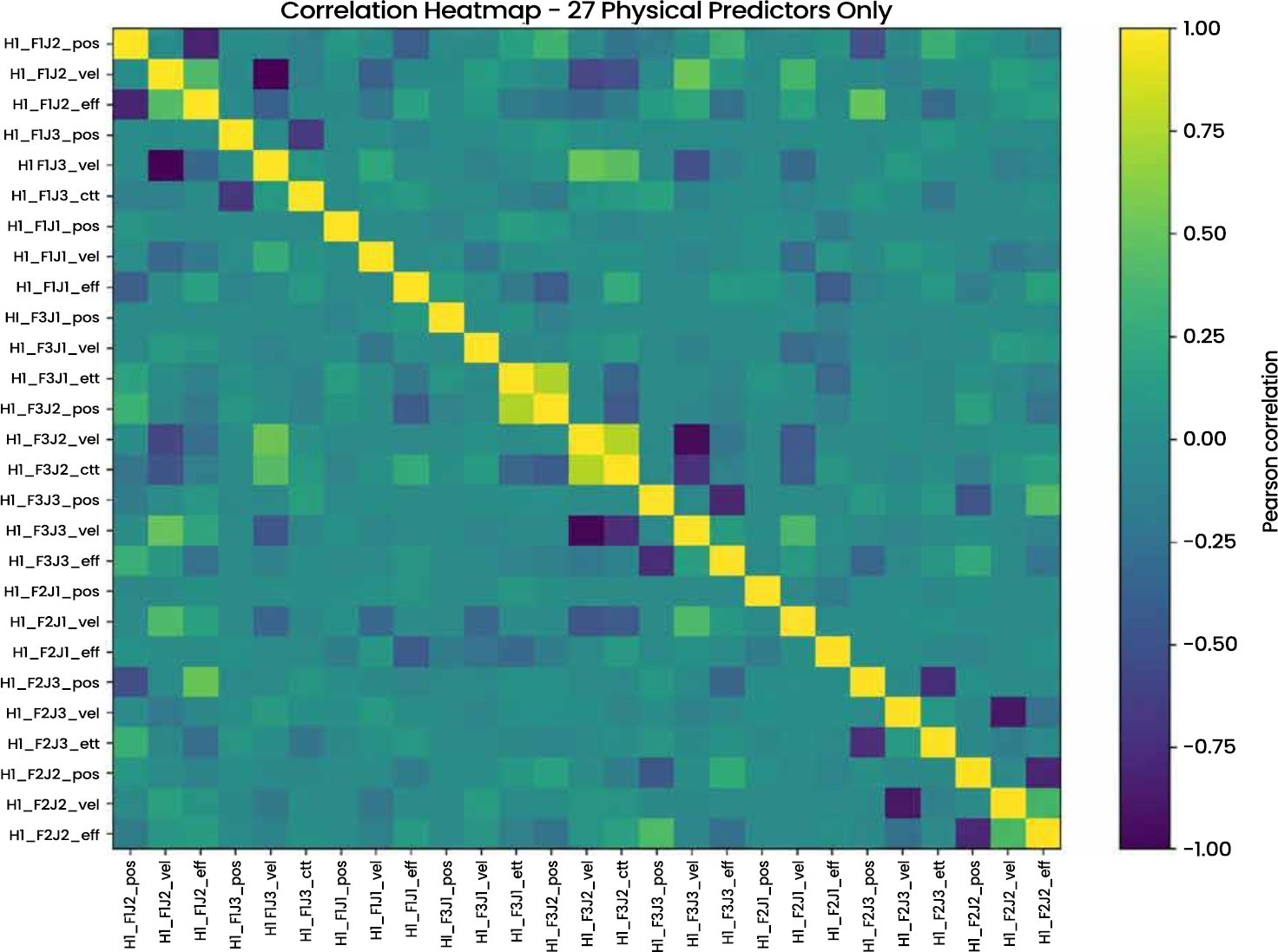
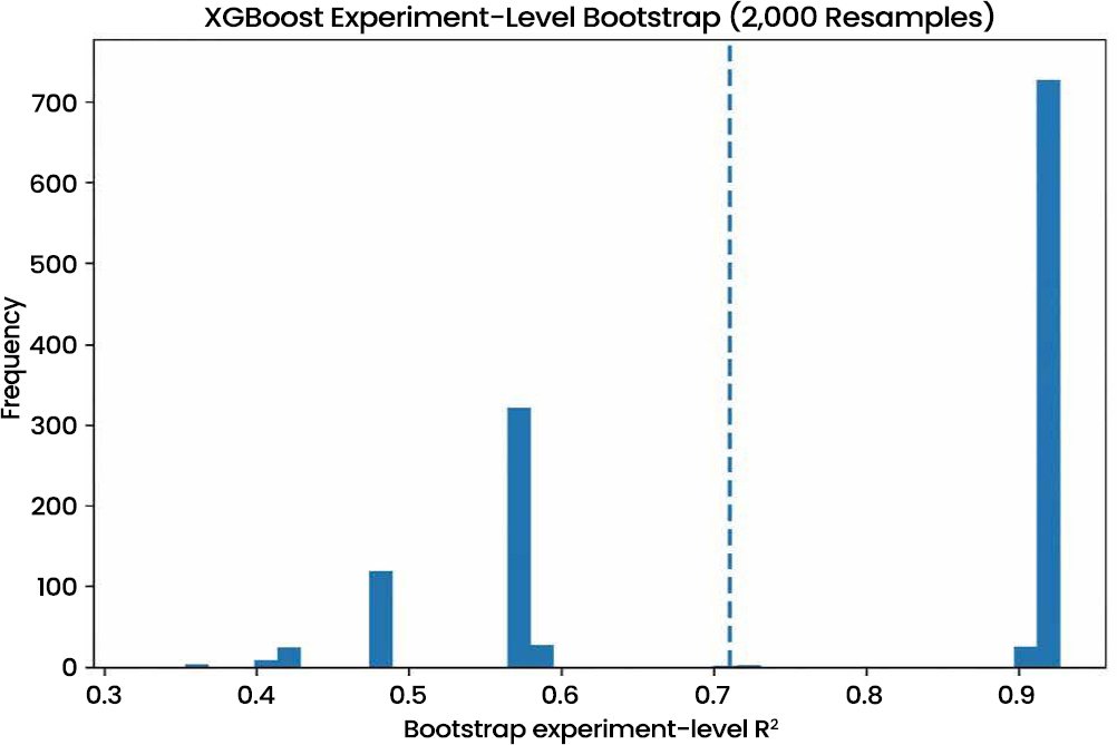
Fig. (2). Identifier-free correlation heatmap of the 27 physical proprioceptive variables.

Fig. (3) shows the experiment-level XGBoost bootstrap distribution from 2,000 resamples of the held-out experiment predictions. Resampling was performed over unique experiments, so each grasp experiment, rather than each measurement row, is the sampling unit. The corresponding 95% bootstrap interval for XGBoost R² is 0.4809–0.9227; Table 6 reports the experiment-level bootstrap intervals for all models. The interval reflects finite held-out-experiment sampling uncertainty for the fixed fitted model and does not represent a model-refitting bootstrap.

Fig. (3). Experiment-level bootstrap distribution of R² (2,000 Resamples).

3.6. Retrospective Analysis Framework

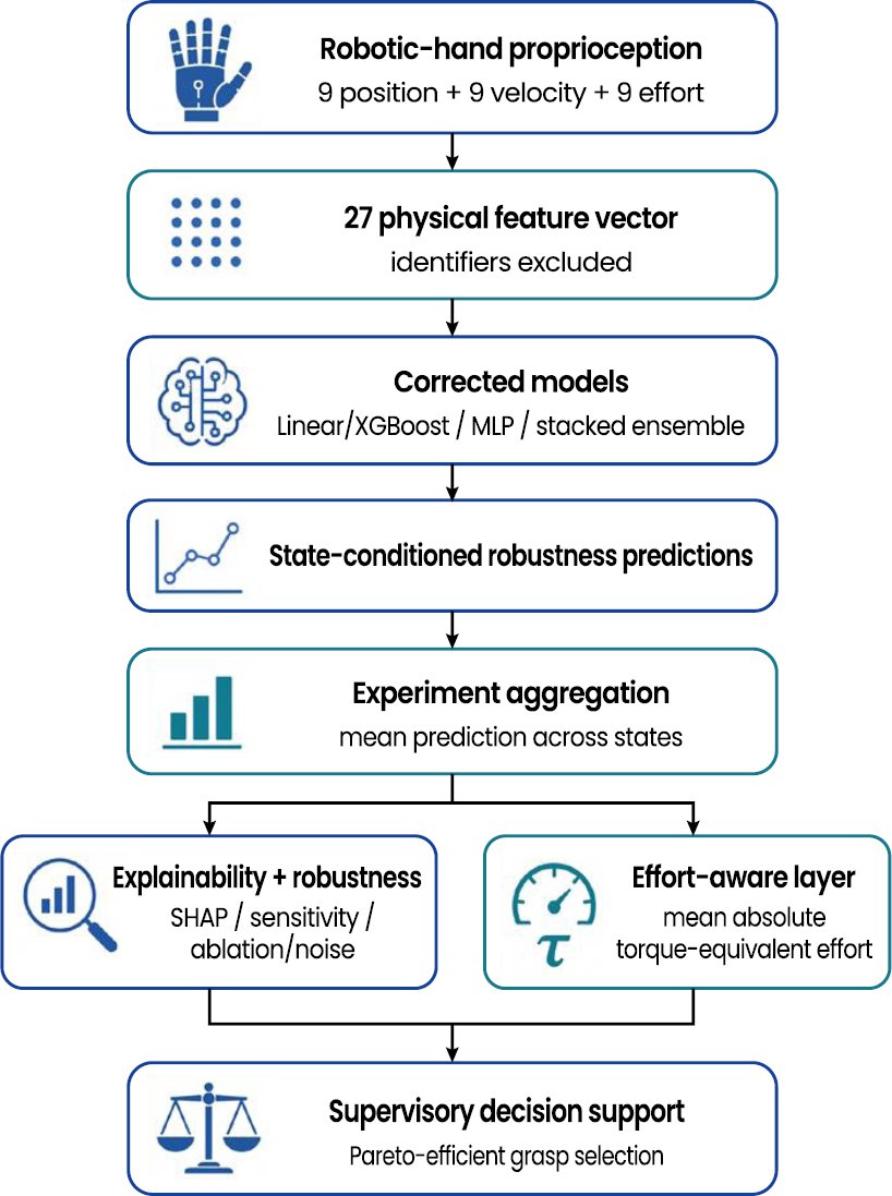
Fig. (4) summarises the analysis flow. The 27 physical channels feed identifier-free state-conditioned models; all recorded states in a completed episode are aggregated to one experiment-level robustness estimate. In parallel, mean absolute effort is calculated from all effort channels and states in that episode. Explainability and Pareto analysis then support model auditing and offline robustness–effort comparison.

Fig. (4). Validated retrospective framework for experiment-level robustness prediction and post-episode effort-aware assessment.

4. RESULTS

4.1. Experiment-Level Model Performance

The protocol was executed on 10,788 previously unseen outer-holdout experiments with zero experiment overlap. XGBoost achieved R² = 0.7104, MAE = 9.52, MedAE = 5.11, RMSE = 31.97 and Spearman ρ = 0.915; the stacked ensemble achieved R² = 0.7132, MAE = 9.72, MedAE = 5.14, RMSE = 31.81 and Spearman ρ = 0.913. Thus, stacking improves R² by only 0.0028 and RMSE by 0.16 while worsening MAE by 0.20, so the result should be interpreted as near-equivalence rather than practical dominance of the ensemble (Table 3).

Table 3. Experiment-level model performance on the experiment-disjoint holdout (10,788 experiments).

ModelMAERMSER²
Linear Regression20.5740.350.5386
XGBoost9.5231.970.7104
Neural Network (MLP)12.0534.940.6539
Stacked Ensemble9.7231.810.7132

Extreme-case robustness and the CV/holdout gap. The unstratified outer holdout contains the dataset’s unique maximum target of 2933.58, whereas the largest outer-development target is 335.62. XGBoost predicts 2.29 for this experiment, an absolute error of 2931.29; the case alone contributes 77.95% of the total holdout squared error. Excluding only this observation as a diagnostic sensitivity analysis raises R² from 0.7104 to 0.9183 and reduces RMSE from 31.97 to 15.01, while MedAE remains 5.11 and Spearman ρ remains approximately 0.916. This pattern is reproduced in the five-fold analysis: the four folds whose validation targets remain within the trained range achieve R² = 0.9151–0.9206, whereas the fold that withholds the same 2933.58 case falls to R² = 0.7122 (Table 4). The apparently large CV/holdout difference therefore reflects a rare out-of-range extrapolation condition and different split construction, not broad deterioration on typical grasps. The extreme observation is retained in all primary metrics; its exclusion is reported only for robustness diagnosis.

Table 4. Robust and extreme-case holdout diagnostics for XGBoost and the stacked ensemble.

Evaluation / MetricXGBoostStacked Ensemble
Full holdout R²0.71040.7132
Full holdout MAE9.529.72
Full holdout MedAE5.115.14
Full holdout RMSE31.9731.81
Full holdout Spearman ρ0.9150.913
R² excluding only target = 2933.58 (sensitivity)0.91830.9227
RMSE excluding only target = 2933.58 (sensitivity)15.0114.60

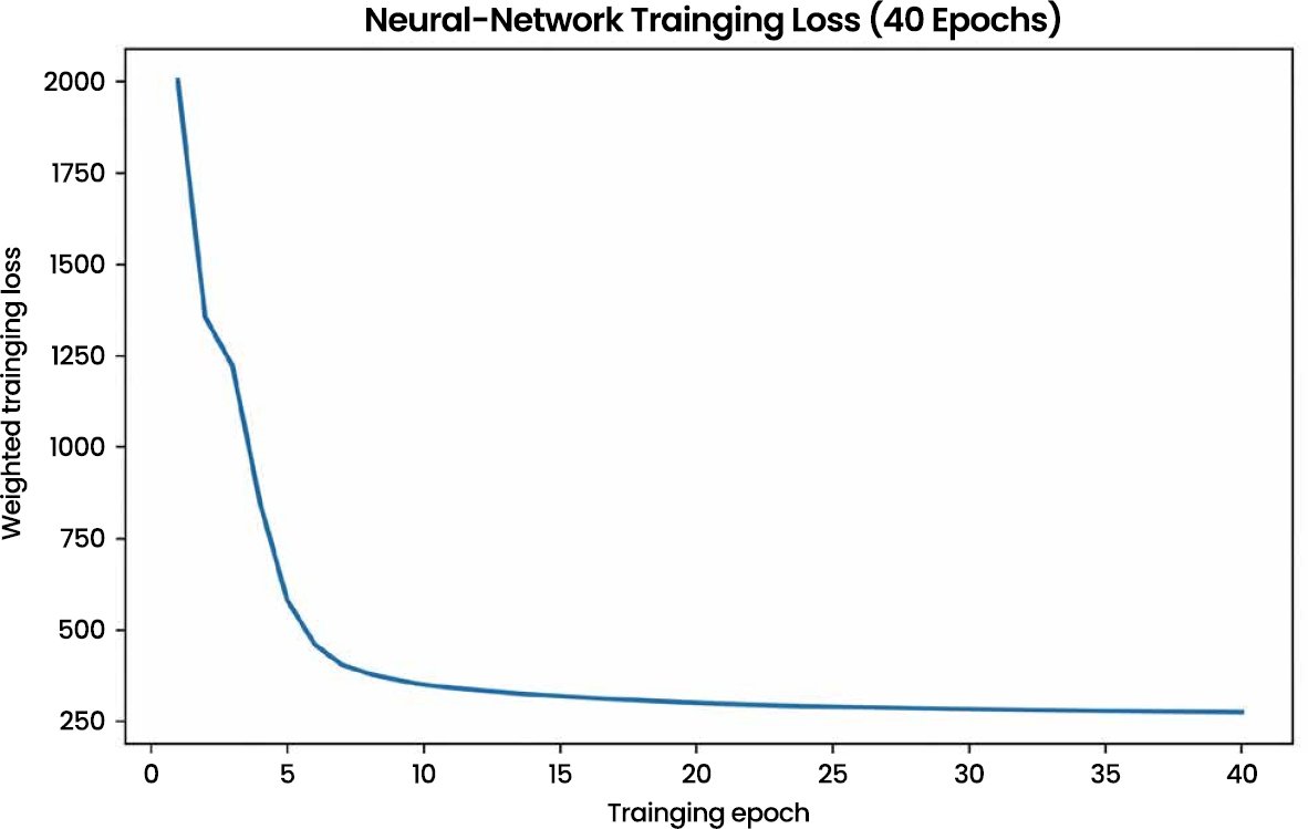
Fig. (5) documents convergence of the weighted MLP training run. The curve is a training diagnostic only; model generalisation is established separately by experiment-disjoint holdout and cross-validation metrics.

Fig. (5). MLP training loss across 40 Epochs.

4.2. Identifier-Free Feature Importance & Explainability

All explainability analyses were regenerated from the XGBoost model using only the 27 physical predictors; measurement_number and experiment_number were excluded from X. SHAP values, gain importance, sensitivity and ablation describe how the fitted model relies on recorded joint states when estimating the released robustness target.

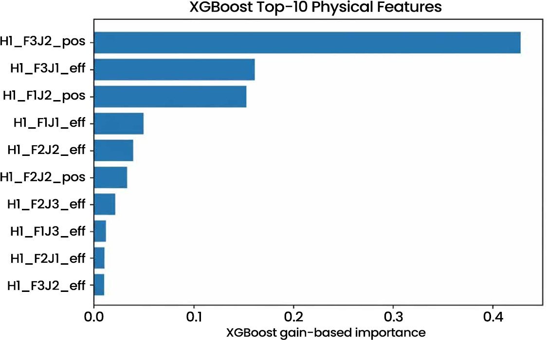
Fig. (6) shows H1_F3J2_pos as the largest XGBoost split-based importance, followed by several effort and position channels. Because the identifiers are absent, the ranking reflects the fitted physical predictor set rather than bookkeeping structure.

Fig. (6). XGBoost Top-10 feature importance (Identifiers Excluded).

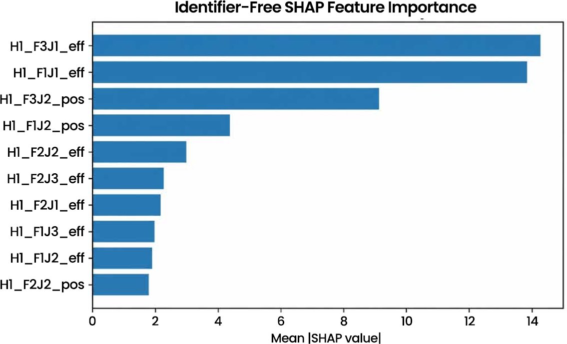
Fig. (7) ranks mean absolute SHAP values on 1,000 held-out measurement states sampled with seed 42. H1_F3J1_eff and H1_F1J1_eff have the largest mean |SHAP| values (14.28 and 13.84), followed by H1_F3J2_pos (9.13) and H1_F1J2_pos (4.38). The result supports a joint role for effort and configuration channels in the model.

Fig. (7). Global SHAP importance for the identifier-free XGBoost model.

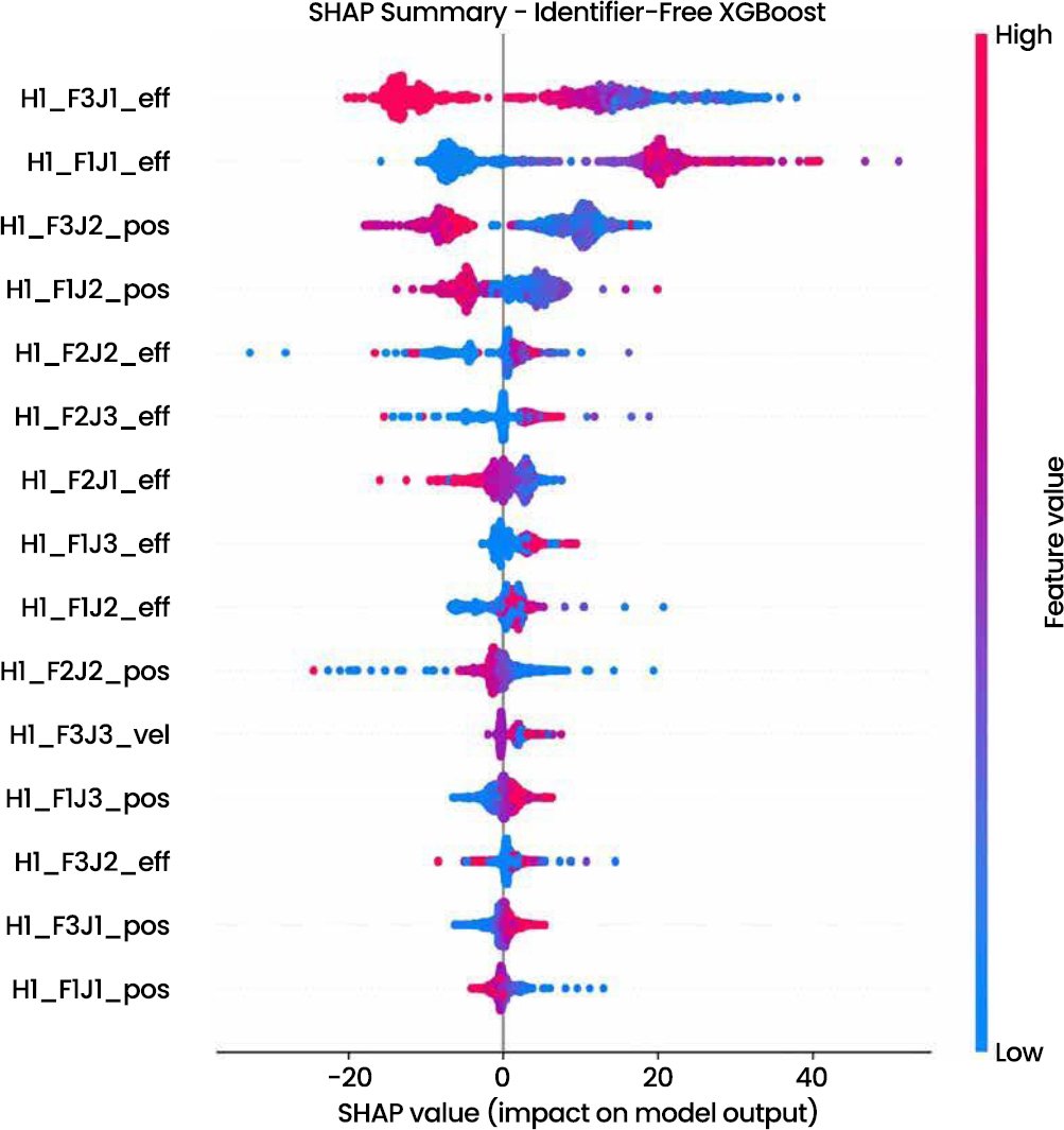
Fig. (8) visualises the direction and magnitude of SHAP contributions across the held-out sample. The distribution shows nonlinear and heterogeneous model associations among effort and position channels without relying on experiment_number or measurement_number.

Fig. (8). SHAP summary plot for the 27-channel XGBoost model.

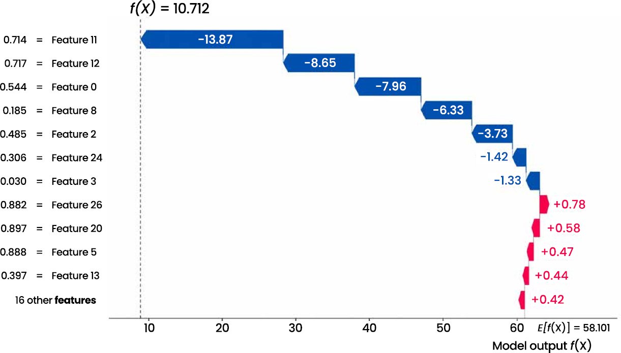
Fig. (9) provides an instance-level explanation from the identifier-free XGBoost model and illustrates how the selected physical state contributes to the model output.

Fig. (9). Local SHAP explanation for a held-out measurement state.

Across Figs. (6–9), the physically supportable conclusion is limited to associations between measured joint configuration, motion, actuator effort and the released experiment-level robustness target. No direct inference about material intelligence, deformation or compliance is made.

4.3. Experiment-Level Generalisation, Timing and Dataset Structure

The analyses distinguish repeated measurement states from independent grasp outcomes. State-conditioned estimates are generated for individual rows, while the reported experiment-level value averages all states recorded in a completed episode. The following figures therefore describe experiment-level behaviour and dataset structure.

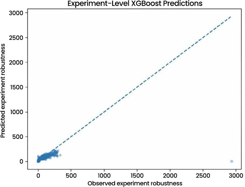
Fig. (10) compares one retrospective prediction per held-out experiment with its released robustness target. The target of 2933.58 is 8.74 times the outer-development maximum (335.62) and is severely underpredicted by XGBoost (2.29). This single experiment contributes 77.95% of XGBoost holdout squared error. Its presence explains why full-holdout R² is 0.7104 even though most observations follow the principal prediction trend and the holdout R² rises to 0.9183 when this one out-of-range case is excluded only for sensitivity analysis.

Fig. (10). XGBoost: experiment-level actual versus predicted robustness.

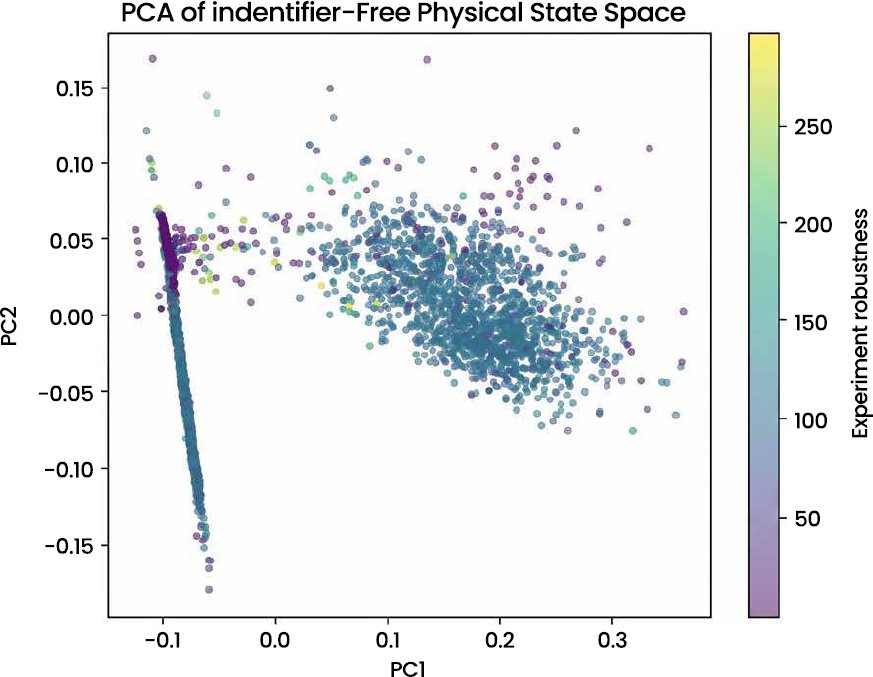
Fig. (11) provides a descriptive two-dimensional projection of the 27 physical channels after identifiers are excluded. PCA is used only for visualisation; no claim of discrete clusters or temporal adaptation is made.

Fig. (11). Identifier-free PCA projection of physical grasp-state space.

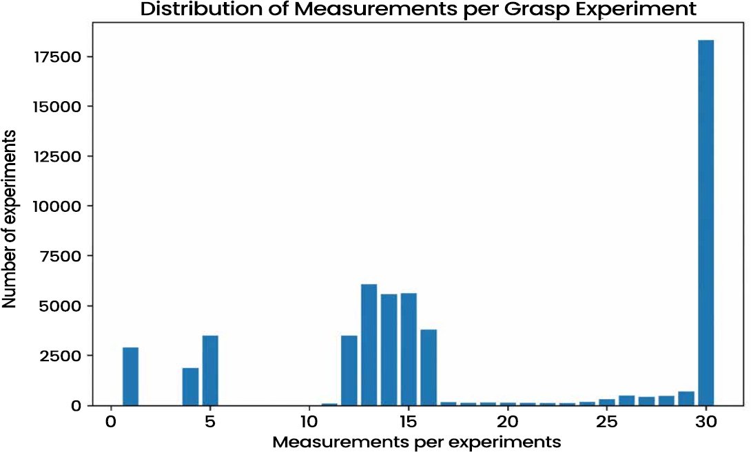
Fig. (12) directly documents the unequal repeated-measurement structure: experiments contain 1–30 rows, with median 15 and a substantial mass at the maximum of 30. This empirical variation motivates the inverse experiment-size weights used in the training objective.

Fig. (12). Distribution of measurement counts per grasp experiment.

4.4. Retrospective Effort–Robustness Trade-offs

The effort trade-off is computed from completed held-out experiments. Estimated robustness is the full-episode aggregate, while mean absolute effort is calculated from all effort channels and recorded states in the same episode. The Pareto layer is therefore an offline comparison. Because the dataset lacks time-integrated electrical power, the analysis is not described as measured energy efficiency.

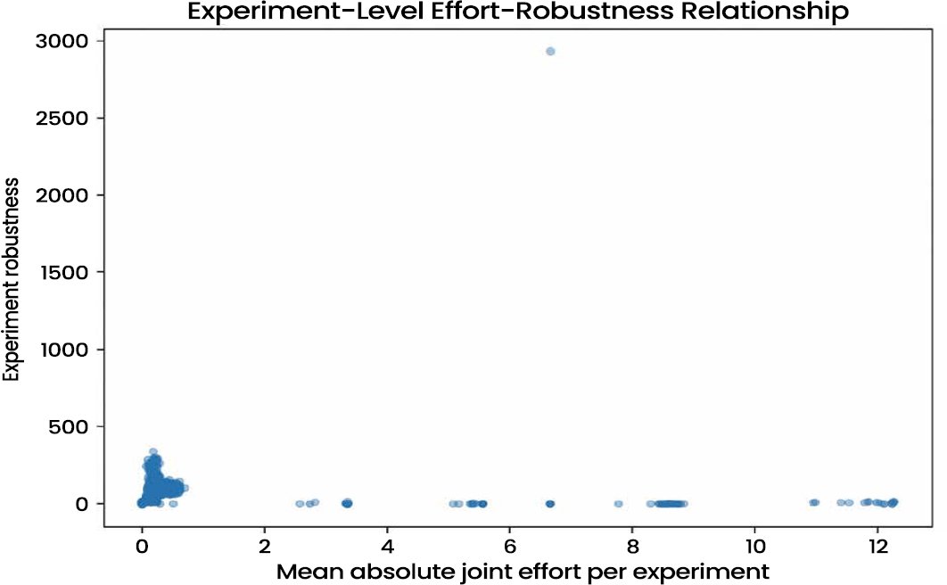
Fig. (13) relates released robustness to the post-episode mean absolute joint-effort descriptor calculated across all effort channels and states in each completed held-out experiment. Using absolute effort prevents positive and negative torque-equivalent channels from cancelling; the descriptor is not available before the full episode has been observed.

Fig. (13). Retrospective experiment-level mean absolute actuation effort versus grasp robustness.

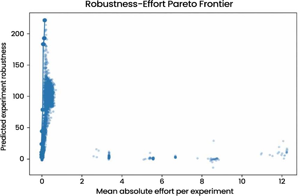
Fig. (14) identifies 12 non-dominated completed held-out experiments under Equation (3). These points summarise offline robustness–effort trade-offs in the observed simulation data; they are not candidate grasps selected prospectively before execution.

Fig. (14). Retrospective experiment-level Pareto frontier for the robustness–effort trade-off.

Fig. (15) shows the independent-unit target distribution rather than the unstable robustness/effort ratio used previously. The strong upper tail (skewness = 3.385) and unique extreme target of 2933.58 are evident and provide context for the sensitivity of RMSE and R² to rare extrapolation cases.

Fig. (15). Experiment-level distribution of the released robustness target.

4.5. Target-Stratified Experiment-Disjoint Stability & CV/Holdout Gap Analysis

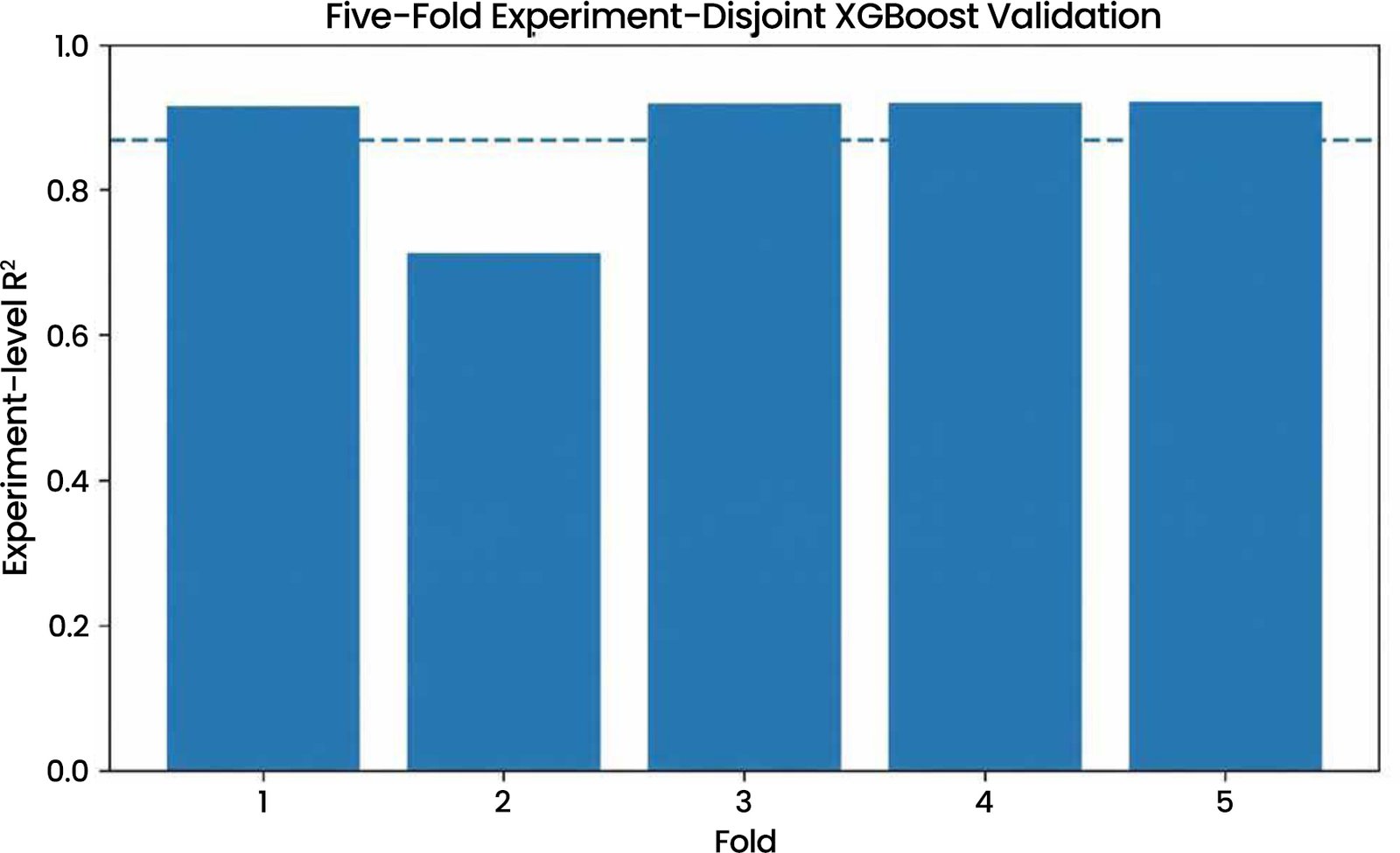
This analysis is separate from the GroupKFold procedure used to train the stack. All 53,937 experiment IDs were stratified by experiment-level target decile and assigned to five folds, with a fresh MinMaxScaler fitted inside each training fold. XGBoost achieved fold R² values of 0.9151, 0.7122, 0.9193, 0.9202 and 0.9206 (mean 0.8775 ± 0.0924), with pooled OOF R² = 0.8687, MAE = 9.46 and RMSE = 19.54 (Table 5). Crucially, the unique target 2933.58 is withheld from training only in Fold 2, where R² = 0.7122; in the other four folds that case is available during training and validation maxima remain within 301.76–338.38, giving R² = 0.9151–0.9206. The outer holdout creates the same extrapolation problem as Fold 2 because 2933.58 is entirely unseen while the development maximum is 335.62, yielding R² = 0.7104. Pooled CV and outer-holdout R² therefore estimate performance under different target-range conditions and should not be treated as contradictory.

Table 5. Target-decile-stratified five-fold experiment-disjoint XGBoost stability analysis.

FoldR²MAERMSE
10.91519.5215.26
20.71229.5731.85
30.91939.4514.97
40.92029.3314.85
50.92069.4214.75
Mean ± SD0.8775 ± 0.09249.46 ± 0.0918.34 ± 7.56
Pooled out-of-fold0.86879.4619.54

The marginal 2,000-resample experiment bootstrap gives XGBoost R² 95% interval 0.481–0.923 and stacked R² interval 0.482–0.927. The 5,000-resample paired bootstrap directly compares the same held-out experiments and gives stacked-minus-XGBoost ΔR² = +0.00285 (95% CI +0.00088 to +0.00514), ΔMAE = +0.2058 (+0.1451 to +0.2657) and ΔRMSE = −0.1575 (−0.4797 to −0.0436) (Table 6). With 10,788 paired experiments these small differences are statistically detectable, but their practical magnitudes are minor and their directions disagree: the stack slightly improves R²/RMSE while slightly worsening MAE. It therefore has no uniform performance advantage over the simpler XGBoost model.

Table 6. Experiment-level and paired bootstrap uncertainty on the outer holdout.

QuantityPoint Estimate95% Bootstrap Interval
Linear Regression R²0.53860.365–0.709
Neural Network (MLP) R²0.65390.438–0.858
XGBoost R²0.71040.481–0.923
Stacked Ensemble R²0.71320.482–0.927
ΔR² (Stack − XGBoost)+0.00285+0.00088 to +0.00514
ΔMAE (Stack − XGBoost)+0.2058+0.1451 to +0.2657
ΔRMSE (Stack − XGBoost)−0.1575−0.4797 to −0.0436

Fig. (16) visualises the target-stratified experiment-disjoint stability results. Fold 2 is the only fold in which the unique 2933.58 experiment is withheld from training, and its R² = 0.7122 closely matches the outer-holdout R² = 0.7104, where the same target is also unseen during training. The remaining four folds include that case in training and evaluate only within the ordinary target range, producing R² values near 0.92.

Fig. (16). Five-fold experiment-level XGBoost R².

4.6. Sensitivity, Ablation & Synthetic Noise Stress Testing

Sensitivity, feature-group ablation and sensor-noise analyses were rerun with the identifier-free XGBoost model. We now define the perturbation magnitude and resampling seeds explicitly, and we calculate all reported R² values after averaging predictions within held-out experiments (Table 7).

Table 7. Sensitivity analysis (+0.01 on the normalised feature scale).

FeatureMean |Δ prediction|
H1_F1J1_eff36.57
H1_F2J1_eff10.41
H1_F1J2_eff8.33
H1_F1J3_eff7.15
H1_F1J3_pos6.43

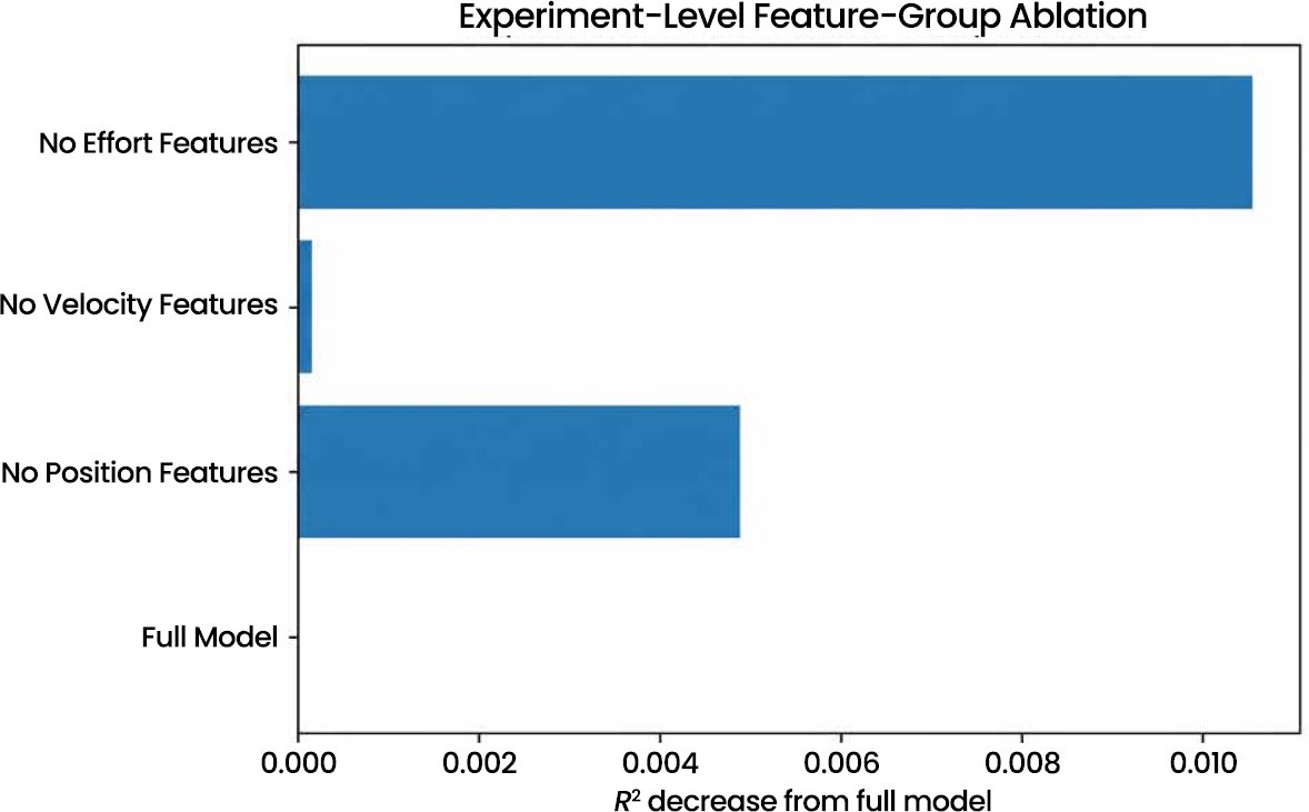
The ablation results show modest but interpretable group effects. Removing effort causes the largest decline in experiment-level R² (−0.0105), followed by position (−0.0049), while removing velocity changes R² by only −0.0001. These values do not justify describing any single channel group as independently essential (Table 8).

Table 8. Experiment-level feature-group ablation results.

Model VariantExperiment R²Δ R²
Full XGBoost0.71040.0000
No Position Features0.7055−0.0049
No Velocity Features0.7102−0.0001
No Effort Features0.6998−0.0105

Fig. (17) visualises the same ablation comparison. The relatively small losses show that information is distributed across multiple physical channel groups, with the strongest measured decrement arising after effort removal.

Fig. (17). Experiment-level feature-group ablation.

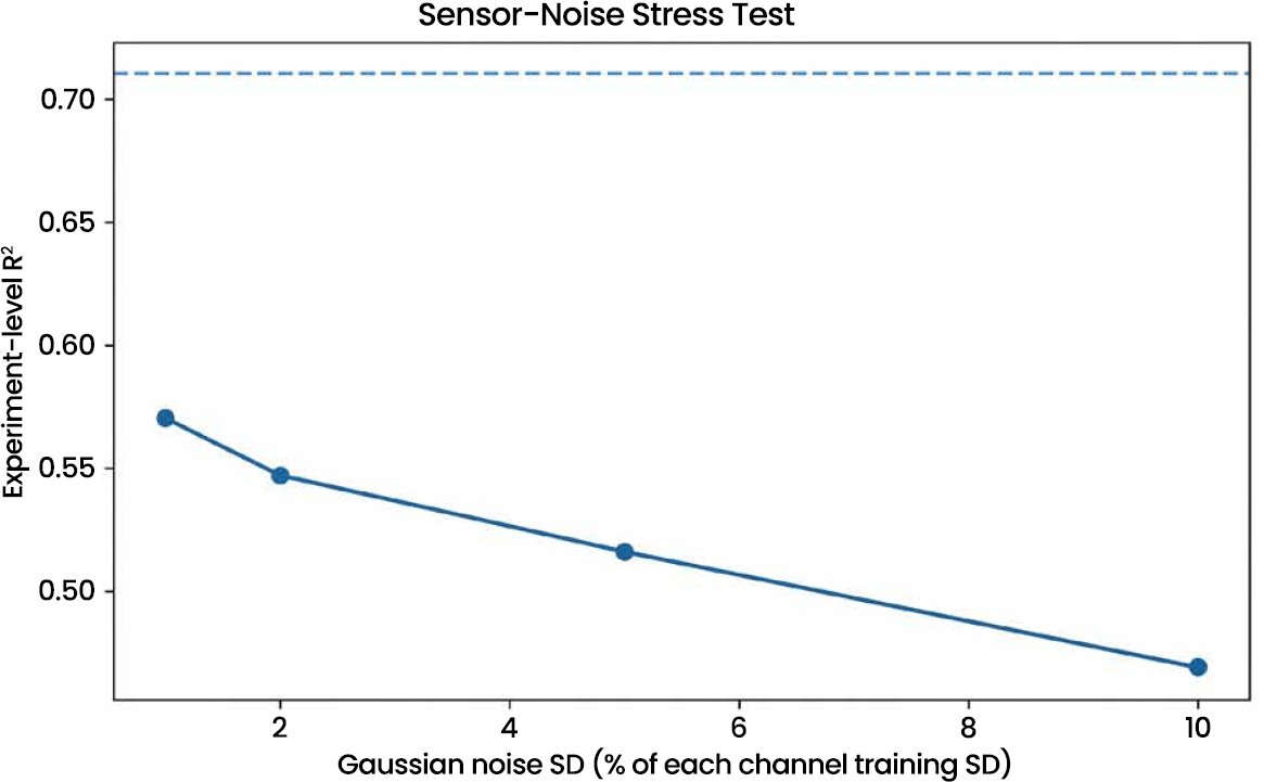
Fig. (18) reports a model-level perturbation stress test, not a validation of physical sensors. After independent Gaussian noise scaled to each channel’s development-set SD, mean experiment-level R² decreases from the baseline 0.7104 to 0.5704 ± 0.0011 at 1% relative noise, 0.5471 ± 0.0010 at 2%, 0.5159 ± 0.0011 at 5% and 0.4686 ± 0.0013 at 10%. The monotonic degradation shows that the fitted predictor is sensitive to synthetic measurement perturbations. Because no hardware sensor specification, calibration trace, fault model, or real-sensor experiment is available, these results do not establish sensor accuracy, reliability, tolerance, or physical noise robustness.

Fig. (18). Synthetic noise stress test of model predictions (not hardware sensor validation).

4.7. Computational Efficiency

Table 9 reports computational throughput of the XGBoost model in the current CPU environment. A 1,000-state batch was timed over 100 repetitions after warm-up. The result is a throughput benchmark only and must not be interpreted as end-to-end controller latency.

Table 9. Computational throughput of the XGBoost model (CPU; Not End-to-End control latency).

MetricValue
Mean batch inference time0.001548 s
Throughput-equivalent per-state time0.001548 ms
Equivalent throughput≈645,983 states/s
Inference batch size1,000 states
Timing repetitions100

Mean batch inference time was 0.001548 s for 1,000 states, corresponding to a throughput-equivalent 0.001548 ms per state (approximately 645,983 states/s). This is a state-level computational throughput measure and does not include episode accumulation or experiment-level aggregation.

4.8. Deployment Requirements

Translation to prospective online and physical deployment would require fixed-prefix or rolling-trajectory evaluation, a contemporaneous effort estimate, time-indexed data separation, pre-specified decision thresholds, calibrated sensing, end-to-end latency measurement and prospective closed-loop validation.

5. DISCUSSION

The lower outer-holdout R² relative to pooled five-fold validation is best interpreted as reflecting target-range shift and extrapolation difficulty rather than broad deterioration in model performance. Robust diagnostics such as MedAE and Spearman ρ remain comparatively stable, while the detailed extreme-case analysis in Section 4.1 shows why squared-error metrics are more sensitive to the rare out-of-range observation.

5.1. Interpretation of Results

Identifier-free analyses show that effort and position channels are prominent in the fitted XGBoost model: global SHAP ranks H1_F3J1_eff and H1_F1J1_eff highest, and effort-group ablation produces the largest R² decrease (−0.0105). These attributions describe model associations and should not be interpreted as causal joint mechanics or evidence that intervening on a high-SHAP variable would improve grasp robustness.

The available data support interpretation in terms of joint configuration, joint motion and actuator effort. They do not directly support a two-stage material-compliance mechanism. Any discussion of compliant morphology is therefore framed as an external engineering hypothesis that requires dedicated measurements of deformation, contact, stiffness or material state.

The MLP improves on Linear Regression but remains below XGBoost and stacking on the full held-out experiment set. Paired bootstrap differences are small and metric-dependent, so the stacked ensemble offers little practical benefit relative to the more parsimonious XGBoost model.

5.2. Relation to Compliance and Material-Intelligence Research

Compliance and material-intelligence research provide a useful wider context because physical morphology can contribute to successful manipulation [31, 32]. The present benchmark, however, contains no direct measurements of material composition, stiffness, constitutive parameters, strain, deformation fields or distributed soft-body dynamics. The current results therefore do not constitute experimental evidence of material intelligence. At most, the proposed predictor could later be integrated with compliant or soft robotic systems if validated using appropriate material and physical-sensing variables.

The study’s principal contribution is consequently not a new ensemble architecture but an experiment-aware validation framework for this repeated-measurement benchmark. Relative to prior Shadow Smart Grasping classification/failure-prediction studies [9, 38, 39], it combines a continuous experiment-level target, equalised group influence, fold-local preprocessing, explicit CV/holdout range-shift diagnosis, identifier-free explainability, perturbation/ablation checks and effort-aware assessment in one auditable pipeline. This methodological positioning avoids attributing novelty to the underlying XGBoost or stacking algorithms.

THEORETICAL IMPLICATIONS

The experiment-level target distribution and the performance of nonlinear models support nonlinear modelling of the joint-state/robustness relationship, but they do not demonstrate nonlinear material mechanics. Explainability is most defensibly used to audit model reliance on meaningful physical channels. The absence of identifiers from the regenerated SHAP rankings provides a stronger basis for interpretation than the archived identifier-contaminated outputs.

PRACTICAL APPLICATIONS

The analysis supports post-episode robustness assessment of completed grasp episodes. Joint encoder and actuator-feedback measurements are transformed into state-conditioned estimates and aggregated to one experiment-level robustness value, after which observed effort can be summarised for offline comparison. This can support model auditing, dataset analysis and future controller design.

Potential application domains include prosthetic or assistive hands, surgical and rehabilitation manipulation, collaborative industrial robots and warehouse automation. Translation to prospective operation requires partial-trajectory validation, sensing calibration, a contemporaneous effort-cost estimate, middleware integration, end-to-end latency measurement and application-specific safety assessment.

The robustness–effort formulation may inform actuator and grasp-strategy studies by identifying completed episodes that combine higher estimated robustness with lower observed mean absolute effort. Because the benchmark lacks direct material and electrical-energy measurements, claims about material-aware design or reduced electrical energy require additional experiments.

LIMITATIONS AND FUTURE DIRECTION

The main limitations are data-domain and deployment limitations rather than unresolved leakage. The benchmark is simulated, uses a single grasped object, and all confirmatory metrics use complete episodes; consequently, online pre-outcome operation, cross-object generalisation and simulation-to-real transfer remain unvalidated. The provider’s exact robustness-scoring transformation is unavailable. The target distribution also contains one severe range-shift case, making squared-error metrics influence-sensitive; full-set R²/RMSE are therefore interpreted alongside MAE, MedAE, Spearman ρ, fold behaviour and the explicit sensitivity analysis.

The bootstrap intervals are conditional on the already fitted models and omit model-refitting and hyperparameter-selection uncertainty. The synthetic-noise experiment is a model stress test defined relative to empirical channel variability rather than a calibrated hardware sensor-noise model.

Model development used a locked XGBoost configuration (300 trees, depth 6, learning rate 0.05, subsample 0.80, and colsample_bytree 0.80) inherited from the archived exploratory analysis. No corrected outer-holdout outcomes were used to choose these values, and they are not claimed to be optimal. Because the historical configuration was nevertheless developed on the same benchmark family, some model-development optimism may remain. A future nested experiment-grouped search should tune hyperparameters entirely within outer training folds and evaluate them on untouched outer groups.

Physical validation should include real sensor streams, multiple objects and grasp conditions, sensor calibration and failure characterisation, actuator-loading measurements, end-to-end timing and application-specific safety testing. Claims about compliant-material mechanisms additionally require deformation, stiffness, strain or other material-state measurements that are absent from the benchmark.

Future work should evaluate prefix or partial-trajectory estimation using only information available up to a decision time, define a contemporaneous effort cost, test physical robotic platforms and diverse objects, use nested group-aware tuning, compare alternative aggregation strategies and measure end-to-end control latency. Reinforcement learning or adaptive control can then be assessed within a prospectively validated setting.

CONCLUSION

This study presents a leakage-controlled, experiment-level framework for robustness regression on the Shadow Smart Grasping benchmark. Its methodological contribution is to separate complete experiments before preprocessing, equalise training influence across unequal episode lengths, exclude identifiers from modelling and attribution, and combine range-shift diagnostics, bootstrap comparison, identifier-free explainability, ablation and synthetic perturbation testing.

On 10,788 unseen holdout experiments, XGBoost achieved R² = 0.7104 and remained the most parsimonious high-performing model. The stacked ensemble provided no material practical advantage over XGBoost. A rare out-of-range target materially affected squared-error metrics, underscoring the importance of explicit range-shift diagnostics.

Identifier-free attribution, ablation and synthetic perturbation tests provide complementary model-level diagnostics. Future work should prioritise partial-trajectory estimation, prospective effort modelling, nested group-aware tuning, rare-outcome extrapolation, real-robot multi-object validation and physical closed-loop evaluation.

LIST OF ABBREVIATIONS

MLP

=

Multilayer Perceptron

MedAE

=

Median Absolute Error

RL

=

Reinforcement Learning

VLA

=

Vision-Language-Action

AUTHOR’S CONTRIBUTION

A.R. has contributed to the study conceptualization, methodology, data analysis, interpretation of results, and manuscript writing.

ETHICAL APPROVAL & INFORMED CONSENT

This research did not involve human participants or animal studies. Ethical approval was therefore not required.

AVAILABILITY OF DATA AND MATERIALS

The benchmark dataset analysed in this study is publicly available through Kaggle. The analysis code accompanying auditing, experiment-ID-based outer splitting, inverse-size weighting, fold-local preprocessing for stacking and stability cross-validation, model fitting, experiment-level aggregation, bootstrap resampling, explainability, ablation, defined noise stress testing, and retrospective effort–robustness is reported in Section 3.5.

FUNDING

This research received no specific grant from any funding agency in the public, commercial, or not-for-profit sectors.

CONFLICT OF INTEREST

The author declares no conflict of interest.

ACKNOWLEDGEMENTS

The analysis uses a publicly available robotic-grasp dataset together with established open-source scientific-computing and machine-learning libraries. The authors acknowledge the Shadow Robot Smart Grasping dataset contributors and the open-source research community for enabling reproducible methodological development.

DECLARATION OF AI

The author also used Artificial Intelligence (AI) tools to generate the figures included in the manuscript.

REFERENCES

[1] D. P. Murphy, “Robotics in Physical Medicine and Rehabilitation,” 1st ed., Elsevier, 2023,
https://doi.org/10.1016/C2021-0-00176-0

[2] A. Sarker, T. Ul Islam, and M. R. Islam, “A review on recent trends of bioinspired soft robotics: Actuators, control methods, materials selection, sensors, challenges, and future prospects,” Adv. Intell. Syst., vol. 7, no. 3, Art. no. 2400414, 2025,
https://doi.org/10.1002/aisy.202400414

[3] H. Zhang, J. Tang, S. Sun, and X. Lan, “Robotic grasping from classical to modern: A survey,” arXiv preprint arXiv:2202.03631, 2022,
https://doi.org/10.48550/arXiv.2202.03631

[4] N. Dheerthi, A. K. Kumar, S. Sarveswaran, and A. Murugarajan, “A comprehensive analysis of bio-inspired soft robotic arm for healthcare applications,” in Multidisciplinary Applications of AI Robotics and Autonomous Systems, IGI Global Scientific Publishing, pp. 1–23, 2024,
https://doi.org/10.4018/979-8-3693-5767-5.ch001

[5] W. Dou, G. Zhong, J. Cao, Z. Shi, B. Peng, and L. Jiang, “Soft robotic manipulators: Designs, actuation, stiffness tuning, and sensing,” Adv. Mater. Technol., vol. 6, no. 9, Art. no. 2100018, 2021,
https://doi.org/10.1002/admt.202100018

[6] O. Vermesan, A. Bröring, E. Z. Tragos, M. Serrano, D. Bacciu, S. Chessa, C. Gallicchio, A. Micheli, M. Dragone, A. Saffiotti, P. Simoens, F. Cavallo, and R. Bahr, “Internet of robotic things—Converging sensing/actuating, hyperconnectivity, artificial intelligence and IoT platforms,” in Cognitive Hyperconnected Digital Transformation: Internet of Things Intelligence Evolution, O. Vermesan and J. Bacquet, Eds. River Publishers, pp. 97–155, 2017,
https://doi.org/10.13052/rp-9788793609105

[7] Y. Jiang, S. Moseson, and A. Saxena, “Efficient grasping from RGB-D images: Learning using a new rectangle representation,” in 2011 IEEE International Conference on Robotics and Automation (ICRA), IEEE, pp. 3304–3311, 2011,
https://doi.org/10.1109/ICRA.2011.5980145

[8] K. Damak, M. Boujelbene, C. Acun, A. Alvanpour, S. K. Das, D. O. Popa, and O. Nasraoui, “Robot failure mode prediction with deep learning sequence models,” Neural Comput. Appl., vol. 37, pp. 4291–4302, 2025,
https://doi.org/10.1007/s00521-024-10856-1

[9] S. Sabeeh, “Enhancing robotic grasping performance through data-driven analysis,” Misan J. Eng. Sci., vol. 3, no. 1, pp. 134–156, 2024,
https://doi.org/10.61263/mjes.v3i1.78

[10] R. L. Truby, “Designing soft robots as robotic materials,” Acc. Mater. Res., vol. 2, no. 10, pp. 854–857, 2021,
https://doi.org/10.1021/accountsmr.1c00071

[11] Y. Wang, Y. Wang, R. T. Mushtaq, and Q. Wei, “Advancements in soft robotics: A comprehensive review on actuation methods, materials, and applications,” Polymers, vol. 16, no. 8, p. 1087, 2024,
https://doi.org/10.3390/polym16081087

[12] C. Laschi, “Soft robotics,” in Robotics Goes MOOC: Design, B. Siciliano, Ed. Cham, Switzerland: Springer Nature Switzerland, pp. 245–271, 2025,
https://doi.org/10.1007/978-3-319-75823-7_5

[13] J. Su, K. He, Y. Li, J. Tu, and X. Chen, “Soft materials and devices enabling sensorimotor functions in soft robots,” Chem. Rev., vol. 125, no. 12, pp. 5848–5977, 2025,
https://doi.org/10.1021/acs.chemrev.4c00906

[14] J. Muru and A. Rassõlkin, “A scoping review of energy consumption in industrial robotics,” Machines, vol. 13, no. 7, Art. no. 542, 2025,
https://doi.org/10.3390/machines13070542

[15] X. Wang, R. Wei, Z. Chen, H. Pang, H. Li, Y. Yang, Q. Hua, and G. Shen, “Bioinspired intelligent soft robotics: From multidisciplinary integration to next-generation intelligence,” Adv. Sci., vol. 12, no. 32, Art. no. e06296, 2025,
https://doi.org/10.1002/advs.202506296

[16] Q. M. Marwan, S. C. Chua, and L. C. Kwek, “Comprehensive review on reaching and grasping of objects in robotics,” Robotica, vol. 39, no. 10, pp. 1849–1882, 2021,
https://doi.org/10.1017/S0263574721000023

[17] S. Duenser, B. Thomaszewski, R. Poranne, and S. Coros, “Nonlinear compliant modes for large-deformation analysis of flexible structures,” ACM Trans. Graph., vol. 42, no. 2, Art. no. 21, pp. 1–11, 2022,
https://doi.org/10.1145/3568952

[18] Y. Kondratenko, I. Atamanyuk, I. Sidenko, G. Kondratenko, and S. Sichevskyi, “Machine learning techniques for increasing efficiency of the robot’s sensor and control information processing,” Sensors, vol. 22, no. 3, Art. no. 1062, 2022,
https://doi.org/10.3390/s22031062

[19] R. Liu, F. Nageotte, P. Zanne, M. de Mathelin, and B. Dresp-Langley, “Deep reinforcement learning for the control of robotic manipulation: A focussed mini-review,” Robotics, vol. 10, no. 1, Art. no. 22, 2021,
https://doi.org/10.3390/robotics10010022

[20] A. Haskard and D. Herath, “Secure robotics: Navigating challenges at the nexus of safety, trust, and cybersecurity in cyber-physical systems,” ACM Comput. Surv., vol. 57, no. 9, Art. no. 222, pp. 1–48, 2025,
https://doi.org/10.1145/3723050

[21] S. Daryanavard, “Real-time predictive artificial intelligence: Deep reinforcement learning for closed-loop control systems and open-loop signal processing,” Ph.D. dissertation, Univ. Glasgow, Glasgow, U.K., 2024,
https://doi.org/10.5525/gla.thesis.84692

[22] B. Singh, R. Kumar, and V. P. Singh, “Reinforcement learning in robotic applications: A comprehensive survey,” Artif. Intell. Rev., vol. 55, pp. 945–990, 2022,
https://doi.org/10.1007/s10462-021-09997-9

[23] T. Zhang and H. Mo, “Reinforcement learning for robot research: A comprehensive review and open issues,” Int. J. Adv. Robot. Syst., vol. 18, no. 3, pp. 1–22, 2021,
https://doi.org/10.1177/17298814211007305

[24] B. Zitkovich, T. Yu, S. Xu, P. Xu, T. Xiao, F. Xia, et al.,”RT-2: Vision-Language-Action Models Transfer Web Knowledge to Robotic Control,” in Proc. 7th Conf. Robot Learn. (CoRL), Proc. Mach. Learn. Res., vol. 229, pp. 2165–2183, 2023, Available from: https://proceedings.mlr.press/v229/zitkovich23a/zitkovich23a.pdf

[25] D. Ghosh, H. R. Walke, K. Pertsch, K. Black, O. Mees, S. Dasari, et al., “Octo: An open-source generalist robot policy,” in Proc. Robotics: Science and Systems XX (RSS), Delft, The Netherlands, 2024,
https://doi.org/10.15607/RSS.2024.XX.090

[26] M. J. Kim, K. Pertsch, S. Karamcheti, T. Xiao, A. Balakrishna, S. Nair, et al.,”OpenVLA: An open-source vision-language-action model,” in Proc. 8th Conf. Robot Learn. (CoRL), Proc. Mach. Learn. Res., vol. 270, pp. 2679–2713, 2025, Available from: https://proceedings.mlr.press/v270/kim25c.html

[27] Y. Ze, G. Zhang, K. Zhang, C. Hu, M. Wang, and H. Xu, “3D Diffusion Policy: Generalizable visuomotor policy learning via simple 3D representations,” in Proc. Robotics: Science and Systems (RSS) XX, Delft, The Netherlands, 2024,
https://doi.org/10.15607/RSS.2024.XX.067

[28] K. Black, N. Brown, D. Driess, A. Esmail, M. R. Equi, C. Finn, et al.“π₀: A vision-language-action flow model for general robot control,” in Proc. Robotics: Science and Systems XXI (RSS), Los Angeles, CA, USA, 2025,
https://doi.org/10.15607/RSS.2025.XXI.010

[29] R. Firoozi, J. Tucker, S. Tian, A. Majumdar, J. Sun, W. Liu, et al., “Foundation models in robotics: Applications, challenges, and the future,” Int. J. Robot. Res., vol. 44, no. 5, pp. 701–739, 2025,
https://doi.org/10.1177/02783649241281508

[30] K. Kawaharazuka, J. Oh, J. Yamada, I. Posner, and Y. Zhu, “Vision-language-action models for robotics: A review towards real-world applications,” IEEE Access, vol. 13, pp. 162467–162504, 2025,
https://doi.org/10.1109/ACCESS.2025.3609980

[31] N. Zhang, J. Ren, Y. Dong, X. Yang, R. Bian, J. Li, G. Gu, and X. Zhu, “Soft robotic hand with tactile palm-finger coordination,” Nat. Commun., vol. 16, Art. no. 2395, 2025,
https://doi.org/10.1038/s41467-025-57741-6

[32] Y. Zhou, W. S. Lee, Y. Gu, and Y. She, “Tactile-reactive gripper with an active palm for dexterous manipulation,” npj Robot., vol. 4, Art. no. 13, 2026,
https://doi.org/10.1038/s44182-026-00079-y

[33] C. Özkurt, “Machine learning with industrial robots: Exploring the impact of joint angles on Cartesian coordinates using explainable AI,” Evol. Intell., vol. 18, Art. no. 22, 2025,
https://doi.org/10.1007/s12065-024-01006-6

[34] Z. Xie, X. Liang, and C. Roberto, “Learning-based robotic grasping: A review,” Front. Robot. AI, vol. 10, Art. no. 1038658, 2023,
https://doi.org/10.3389/frobt.2023.1038658

[35] R. Newbury, M. Gu, L. Chumbley, A. Mousavian, C. Eppner, J. Leitner, et al., “Deep learning approaches to grasp synthesis: A review,” IEEE Trans. Robot., vol. 39, no. 5, pp. 3994–4015, 2023,
https://doi.org/10.1109/TRO.2023.3280597

[36] A. Depierre, E. Dellandréa, and L. Chen, “Jacquard: A large-scale dataset for robotic grasp detection,” in Proc. 2018 IEEE/RSJ Int. Conf. Intell. Robots Syst. (IROS), Madrid, Spain, pp. 3511–3516, 2018,
https://doi.org/10.1109/IROS.2018.8593950

[37] E. Jang, A. Irpan, M. Khansari, D. Kappler, F. Ebert, C. Lynch, et al., “BC-Z: Zero-shot task generalization with robotic imitation learning,” in Proc. 5th Conf. Robot Learn. (CoRL), Proc. Mach. Learn. Res., vol. 164, pp. 991–1002, 2022, Available from: https://proceedings.mlr.press/v164/jang22a/jang22a.pdf

[38] A. Alvanpour, C. Acun, K. Spurlock, C. K. Robinson, S. K. Das, D. O. Popa, and O. Nasraoui, “Comparative analysis of post hoc explainable methods for robotic grasp failure prediction,” Electronics, vol. 14, no. 9, Art. no. 1868, 2025,
https://doi.org/10.3390/electronics14091868

[39] C. Acun, A. Ashary, D. O. Popa, and O. Nasraoui, “Optimizing local explainability in robotic grasp failure prediction,” Electronics, vol. 14, no. 12, Art. no. 2363, 2025,
https://doi.org/10.3390/electronics14122363

LIMITATIONS

This study has several limitations. First, the empirical evaluation is based on METR-LA only. Although METR-LA is a widely used benchmark, validation on additional datasets such as PEMS-BAY would strengthen the generalisability of the findings. Second, the statistical analysis is limited by the use of five random seeds. The paired seed-level comparisons are therefore interpreted as exploratory and directional rather than definitive statistical proof. Third, the learned adaptive adjacency matrix provides graph-level transparency, but it does not fully explain individual predictions. Future work should include node-level attribution, temporal attention analysis or counterfactual graph perturbation to support stronger interpretability claims. Fourth, the model was evaluated in an offline forecasting setting and was not deployed in a real-time traffic-management environment. Runtime and inference measurements provide useful computational evidence, but operational deployment would require additional testing under streaming data conditions. Finally, the model’s performance may be sensitive to static graph construction, sparsity strength and missing-value treatment; broader sensitivity analysis would further improve robustness.

CONCLUSION

This study presented a static-adaptive graph attention Transformer model for METR-LA traffic-speed forecasting. The model integrates a static graph prior, adaptive graph learning, local graph diffusion, global spatial attention, Transformer-based temporal encoding and L1 graph sparsity regularisation. The main finding is that combining structural graph information with learned adaptive connectivity provides a technically coherent approach for modelling traffic-speed dynamics over sensor networks. The horizon-wise results suggest that the proposed model maintains lower error across 15-, 30- and 60-minute forecasting horizons compared with the evaluated baselines. The ablation results further suggest that static-adaptive fusion, local/global spatial encoding, temporal self-attention and graph sparsity each contribute to the observed forecasting behaviour under the selected protocol. However, the findings are interpreted cautiously because the evaluation is limited to one benchmark dataset and five repeated seeds. Future work should extend the evaluation to additional traffic datasets, include stronger statistical power, improve prediction-level interpretability and test the model under real-time deployment conditions.

LIST OF ABBREVIATIONS

ASTGCN

=

Attention-based Spatio-Temporal Graph Convolutional Network

GRUs

=

Gated Recurrent Units

GMAN

=

Graph Multi-Attention Network

RNNs

=

Recurrent Neural Networks

STFGNN

=

Spatio-Temporal Fusion Graph Neural Network

AUTHOR’S CONTRIBUTION

B.B.P. has contributed to the study concept, data collection, analysis, manuscript writing, data collection, writing, and proofreading.

ETHICAL APPROVAL & INFORMED CONSENT

Not applicable.

AVAILABILITY OF DATA AND MATERIALS

The data will be made available on reasonable request by contacting the corresponding author [B.B.P.].

FUNDING

None.

CONFLICT OF INTEREST

The author declares that there is no conflict of interest regarding the publication of this article.

ACKNOWLEDGEMENTS

Declared none.

DECLARATION OF AI

During the preparation of this manuscript, the author utilized ChatGPT exclusively to improve the language, grammar, and readability of the text. All generated suggestions were thoroughly reviewed, verified, and revised by the author as necessary. The author takes full responsibility for the content of the manuscript and affirm its accuracy, originality, and scientific integrity.

REFERENCES

[1] Alsehaimi B, Alzamzami O, Alowidi N, Ali M. An adaptive Spatio-Temporal traffic flow prediction using Self-Attention and Multi-Graph networks. Sensors. 2025 Jan 6; 25(1): 282.
https://doi.org/10.3390/s25010282.

[2] Huo Y, Zhang H, Tian Y, Wang Z, Wu J, Yao X. A spatiotemporal graph neural network with graph adaptive and attention mechanisms for traffic flow prediction. Electronics. 2024 Jan 3; 13(1): 212.
https://doi.org/10.3390/electronics13010212.

[3] Zhang Y, Xu W, Ma B, Zhang D, Zeng F, Yao J, Yang H, Du Z. Linear attention based spatiotemporal multi graph GCN for traffic flow prediction. Scientific Reports. 2025 Mar 10; 15(1): 8249.
https://doi.org/10.1038/s41598-025-93179-y.

[4] Zhang J, Yang Y, Wu X, Li S. Spatio-temporal transformer and graph convolutional networks-based traffic flow prediction. Scientific Reports. 2025 Jul 7; 15(1): 24299.
https://doi.org/10.1038/s41598-025-10287-5.

[5] Chen H, Huang J, Lu Y, Huang J. Multi-scale spatio-temporal graph neural network for urban traffic flow prediction. Scientific Reports. 2025 Jul 23; 15(1): 26732.
https://doi.org/10.1038/s41598-025-11072-0.

[6] Yin X, Yu J, Duan X, Chen L, Liang X. Short-term urban traffic forecasting in smart cities: a dynamic diffusion spatial-temporal graph convolutional network. Complex & Intelligent Systems. 2025 Feb; 11(2): 158.
https://doi.org/10.1007/s40747-024-01769-6.

[7] Albalooshi FA. Advancing Urban Planning with Deep Learning: Intelligent Traffic Flow Prediction and Optimization for Smart Cities. Future Transportation. 2025 Oct 2; 5(4): 133.
https://doi.org/10.3390/futuretransp5040133.

[8] Liu R, Shin SY. A review of traffic flow prediction methods in intelligent transportation system construction. Applied Sciences. 2025 Apr 1; 15(7): 3866.
https://doi.org/10.3390/app15073866.

[9] Li Y, Yu R, Shahabi C, Liu Y. Diffusion convolutional recurrent neural network: Data-driven traffic forecasting. arXiv preprint arXiv:1707.01926. 2017 Jul 6.

[10] Shao Z, Zhang Z, Wei W, Wang F, Xu Y, Cao X, Jensen CS. Decoupled dynamic spatial-temporal graph neural network for traffic forecasting. arXiv preprint arXiv:2206.09112. 2022 Jun 18.
https://doi.org/10.14778/3551793.3551827.

[11] Jiang W, Luo J. Graph neural network for traffic forecasting: A survey. Expert systems with applications. 2022 Nov 30; 207: 117921.
https://doi.org/10.1016/j.eswa.2022.117921.

[12] Bai HY, Liu X. T-Graphormer: using Transformers for spatiotemporal forecasting. arXiv preprint arXiv:2501.13274. 2025 Jan 22.
https://doi.org/10.48550/arXiv.2501.13274.

[13] Guo Z, Lu M, Han J. Temporal graph attention network for spatio-temporal feature extraction in research topic trend prediction. Mathematics. 2025 Feb 20; 13(5): 686.
https://doi.org/10.3390/math13050686.

[14] Cai F, Wang Y, Yu W, Wu J, Liu C, Li XA. ASISTGCRN: A novel approach to traffic prediction using attention-based spatiotemporal graph networks. Proceedings of the Institution of Mechanical Engineers, Part D: Journal of Automobile Engineering. 2025 Nov 27: 09544070251390950.
https://doi.org/10.1177/09544070251390950.

[15] Zhao Y, Li H, Zhou H, Attar HR, Pfaff T, Li N. A review of graph neural network applications in mechanics-related domains. Artificial Intelligence Review. 2024 Oct 4; 57(11): 315.
https://doi.org/10.1007/s10462-024-10931-y.

[16] Yang C, Zhang W, Yingjiang Z. An Overview of Spatiotemporal Network Forecasting: Current Research Status and Methodological Evolution. Mathematics. 2025; 14(1): 18.
https://doi.org/10.3390/math14010018.

[17] Chang J, Yin J, Hao Y, Gao C. STFDSGCN: spatio-temporal fusion graph neural network based on dynamic sparse graph convolution GRU for traffic flow forecast. Sensors. 2025 May 30; 25(11): 3446.
https://doi.org/10.3390/s25113446.

[18] Veličković P, Fedus W, Hamilton WL, Liò P, Bengio Y, Hjelm RD. Deep graph infomax. arXiv preprint arXiv:1809.10341. 2018 Sep 27.
https://doi.org/10.48550/arXiv.1809.10341.

[19] Xiao Z, Shen Q, Li C, Li D, Liu Q. An adaptive spatiotemporal dynamic graph convolutional network for traffic prediction. Scientific Reports. 2025 Jul 25; 15(1): 27098.
https://doi.org/10.1038/s41598-025-12261-7.

[20] Jiang M, Liu Z. Traffic flow prediction based on dynamic graph spatial-temporal neural network. Mathematics. 2023 May 31; 11(11): 2528.
https://doi.org/10.3390/math11112528.

[21] Bai L, Yao L, Li C, Wang X, Wang C. Adaptive graph convolutional recurrent network for traffic forecasting. Advances in neural information processing systems. 2020; 33: 17804-15.

[22] Ma J, Zhao J, Hou Y. Spatial-temporal transformer networks for traffic flow forecasting using a pre-trained language model. Sensors. 2024 Aug 25; 24(17): 5502.
https://doi.org/10.3390/s24175502.

[23] Tang J, Xia L, Huang C. Explainable spatio-temporal graph neural networks. InProceedings of the 32nd ACM International Conference on Information and Knowledge Management 2023 Oct 21 (pp. 2432-2441).
https://doi.org/10.1145/3583780.3614871.

[24] Yan H, Chen D, Jiang G, Wang B, Cao L, Dong J, Yu Y. DGraFormer: Dynamic Graph Learning Guided Multi-Scale Transformer for Multivariate Time Series Forecasting. InProceedings of the Thirty-Fourth International Joint Conference on Artificial Intelligence (IJCAI 2025) 2025 Aug 16 (pp. 3516-3524).
https://doi.org/10.24963/ijcai.2025/391.

[25] Remmouche B, Boukraa D, Zakharova A, Bouwmans T, Taffar M. Long-term spatio-temporal graph attention network for traffic forecasting. Expert Systems with Applications. 2025 Sep 1; 288: 128244.
https://doi.org/10.1016/j.eswa.2025.128244.

[26] Feng A, Tassiulas L. Adaptive graph spatial-temporal transformer network for traffic forecasting. InProceedings of the 31st ACM international conference on information & knowledge management 2022 Oct 17 (pp. 3933-3937).
https://doi.org/10.1145/3511808.3557540.

[27] El-Meehy AO, El-Kharbotly AK, El-Beheiry MM. Systematic hyperparameter analysis of GRU and LSTM across demand pattern types: A demand-characteristic-driven meta-learning framework for rapid optimization. Scientific Reports. 2025 Dec 25.
https://doi.org/10.1038/s41598-025-31508-x.

[28] Huang X, Wang J, Lan Y, Jiang C, Yuan X. MD-GCN: A multi-scale temporal dual graph convolution network for traffic flow prediction. Sensors. 2023 Jan 11; 23(2): 841.
https://doi.org/10.3390/s23020841.

[29] Singh V, Sahana SK, Bhattacharjee V. Integrated spatio-temporal graph neural network for traffic forecasting. Applied Sciences. 2024 Dec 10; 14(24): 11477.
https://doi.org/10.3390/app142411477.

[30] He S, Luo Q, Du R, Zhao L, He G, Fu H, Li H. STGC-GNNs: A GNN-based traffic prediction framework with a spatial-temporal Granger causality graph. Physica A: Statistical Mechanics and its Applications. 2023 Aug 1; 623: 128913.
https://doi.org/10.1016/j.physa.2023.128913.

[31] Vrahatis AG, Lazaros K, Kotsiantis S. Graph attention networks: a comprehensive review of methods and applications. Future Internet. 2024 Sep 3; 16(9): 318.
https://doi.org/10.3390/fi16090318.

[32] Zhu Y. Graph neural networks for urban traffic flow forecasting: A comprehensive review and future perspectives. 2025.
https://doi.org/10.54254/2753-8818/2025.DL27990.

[33] Zong X, Guo J, Liu F, Yu F. TSTA-GCN: trend spatio-temporal traffic flow prediction using adaptive graph convolution network. Scientific Reports. 2025 Apr 18; 15(1): 13449.
https://doi.org/10.1038/s41598-025-96833-7.

[34] Dai BA, Ye BL, Li L. A novel hybrid time-varying graph neural network for traffic flow forecasting. arXiv preprint arXiv:2401.10155. 2024 Jan 17.
https://doi.org/10.48550/arXiv.2401.10155.

[35] Wei S, Yang Y, Liu D, Deng K, Wang C. Transformer-based spatiotemporal graph diffusion convolution network for traffic flow forecasting. Electronics. 2024 Aug 9; 13(16): 3151.
https://doi.org/10.3390/electronics13163151.

[36] Kwak S. PEMS-BAY and METR-LA in csv. Zenodo. 2020.
https://doi.org/10.5281/zenodo.5146275.

Insert math as
Block
Inline
Additional settings
Formula color
Text color
#333333
Type math using LaTeX
Preview
\({}\)
Nothing to preview
Insert