Article ID: PD2601202006
Views: 202A Hybrid Physics-Informed Deep Learning Framework for Robust Multivariate System Modelling Under Uncertainty – Copy
 PDF
PDF
⬇ Downloads: 15
1. INTRODUCTION
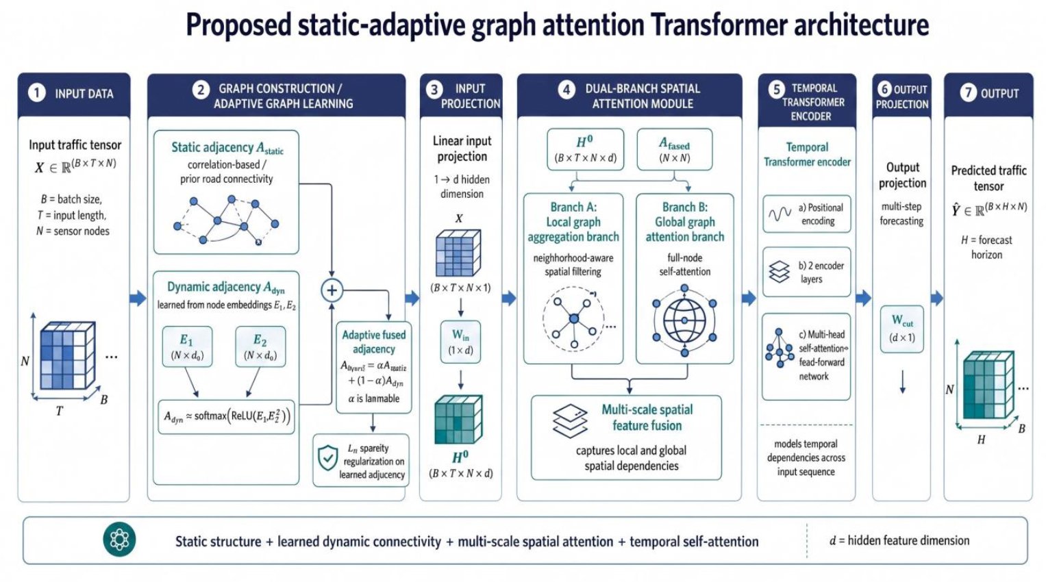
Urban mobility systems produce large-scale sensor streams that are spatially dependent and temporally dynamic. A speed change at one freeway sensor may propagate to downstream sensors, while recurring daily patterns, incidents and capacity fluctuations alter the temporal profile of each node [1, 2, 3]. This makes traffic forecasting a graph time-series problem rather than an ordinary univariate prediction task. In this setting, a road network can be represented as G = (V, E, A), where V denotes the sensor nodes, E denotes the edges or relationships between sensors, and A denotes the adjacency matrix used to control spatial message passing [4].
Traditional recurrent and convolutional time-series models can learn temporal trends but often ignore the topology of the transportation network [5, 6]. Graph neural networks address this gap by allowing each sensor to aggregate information from other sensors through a graph structure. However, the graph used by many early models is fixed and is usually based on road distance, physical connectivity or expert assumptions. Such assumptions are useful but incomplete because real congestion propagation can change with demand, lane disruptions, time of day and non-recurring events [7, 8].
This paper presents an adaptive attention-driven architecture for graph-based traffic forecasting. The design combines four elements: static-adaptive graph fusion, local graph diffusion, global spatial attention and temporal self-attention. The static graph preserves stable sensor relationships, while the adaptive graph captures hidden sensor dependencies that are not directly encoded by a fixed topology. The local branch learns neighbourhood propagation, and the global branch allows non-neighbouring sensors to influence one another when their speed patterns become correlated. The temporal Transformer encoder then processes each node-specific sequence using self-attention rather than sequential recurrence.
The empirical design is based on METR-LA because it is a recognised benchmark in traffic forecasting. METR-LA contains traffic-speed observations from 207 loop-detector sensors in Los Angeles County at five-minute intervals and has been widely used in graph-based traffic forecasting studies [9, 10]. Unlike a small pilot file with only a few dozen time points, METR-LA provides enough temporal coverage to support a standard 12-step input and 12-step output forecasting setting. The paper therefore focuses on benchmark-ready validation rather than small-sample demonstration.
The main contribution of this study is a technically integrated spatio-temporal forecasting architecture for graph-based traffic-speed prediction. The contribution is defined as technical integration rather than the independent invention of graph neural networks, attention mechanisms, adaptive adjacency learning or Transformer modelling. The proposed framework combines static-adaptive graph fusion, local graph diffusion, global spatial attention and Transformer-based temporal encoding within one controlled forecasting pipeline. This integrated design is evaluated using chronological data splitting, training-only normalisation, fixed-seed repeated reporting, ablation analysis, saved-checkpoint evaluation and horizon-aware reporting at 15-, 30- and 60-minute forecasting horizons. The manuscript therefore positions the work as a controlled technical integration of existing graph-learning and attention-based forecasting principles rather than as a claim that any single component is entirely new.
2. LITERATURE REVIEW
2.1. Traffic Forecasting as Graph Time-Series Learning
Traffic forecasting has shifted from classical statistical modelling to graph-based deep learning because traffic sensors are not independent. Graph-based methods explicitly encode relationships among sensors and allow each node representation to be updated using nearby or correlated nodes. [11] reviewed the field and noted that graph neural networks are well suited to traffic systems because road networks naturally contain graph structures. Graph Transformers are another advancement, which instead of recurrent layers, involves self-attention mechanics to achieve more efficient long-range temporal learning. The study by [12] has proven the potential of the Transformer architectures in the graph-based tasks, where self-attention performs better than the RNN-based models to capture long-range dependencies on the spatio-temporal data. Transformer-based method is also advantageous in terms of parallelisation and scalability that makes it to be more applicable in large scale and real-time traffic forecasting techniques.
The ASTGCN (Attention-based Spatio-Temporal Graph Convolutional Network) of [13] involves the use of spatial and temporal attention to improve the model capacity to learn local and global dependencies. This model uses spatial attention to concentrate on local dependencies in traffic flow data and temporal attention to model long-term trends, which is effective than other methods to use in complex traffic networks to forecast. ASTGCN is a valuable advancement as it introduces multi-head attention to learn more spatio-temporal relationships [14].
Additionally, the Graph Multi-Attention Network (GMAN) by [15] uses multi-head attention to focus on local- and global-scale spatial dependencies at once. GMAN proposes multi-scale attention, which enhances the capacity of the model in containing the heterogeneous traffic characteristics that are very appropriate in real-time forecasting of traffic in the dynamic traffic scenario. Multi-scale attention enables GMAN to be more flexible to different traffic conditions, since it is able to capture the local relationships that are fine-tuned, as well as the large-scale system-wide impacts.
[16] introduced dynamic graph learning in STFGNN (Spatio-Temporal Fusion Graph Neural Network), which is a significant development. This network assumes a dual pathway model that incorporates graph convolutions of spatial and GRUs (Gated Recurrent Units) of temporal dependencies. The combination of space and time characteristics improves the development of intricate interactions of traffic flow data both in space and time and the overall forecasting outcomes [17]. The present study follows this graph time-series view and treats METR-LA as a dynamic multivariate signal defined over a sensor graph.
2.2. Fixed-Topology Spatio-Temporal Graph Models
Early spatio-temporal graph models such as STGCN and DCRNN established the usefulness of graph convolution for traffic prediction. STGCN used graph convolution and temporal convolution to avoid fully recurrent training, while DCRNN represented traffic propagation as a diffusion process over a directed graph [18]. These methods remain important baselines because they combine spatial graph learning with temporal forecasting. [19] suggest that foundational models such as ST-GCN and DCRNN combine graph convolutions with recurrent neural networks (RNNs) to integrate spatial topology and temporal sequences, but most of them use fixed adjacency matrices based on physical distance, road connectivity, or expert knowledge. These fixed topologies do not scale to the dynamism of traffic flows, in which spatial dependencies change over time due to varying patterns, incidents, external forces such as weather, and events. This rigidity causes inefficient representation of changing network forms, which causes reduced prediction performance, especially when there are non-recurring congestion or non-homogeneous urban conditions [20]. However, fixed topology can be restrictive when the true dependence between two sensors changes over time. Published METR-LA results show that fixed or semi-fixed graph baselines still perform competitively, but their errors increase at longer horizons.
2.3. Adaptive Graph Learning and Dynamic Dependency Modelling
Adaptive graph learning addresses the fixed-topology limitation by learning sensor relationships directly from data. [21] proposed AGCRN, which uses node-adaptive parameter learning and data-adaptive graph generation to infer hidden dependencies. [10] introduced D2STGNN, which separates diffusion and inherent components of traffic signals and includes dynamic graph learning. [22] proposed an evolutionary graph neural network that continuously updates a semantic adjacency matrix during training. These models have low structural interpretability, with learned representations being black boxes, making it difficult to analyse what spatial or temporal aspects a prediction is being driven by [23, 24]. These studies motivate the adaptive component of the present architecture, but this paper retains a static prior so that learned edges do not completely ignore physical or correlation-based structure.
2.4. Multi-Scale Spatial Attention
Single-scale aggregation may not be sufficient for traffic networks because congestion may be local in one period and network-wide in another. Multi-scale models attempt to capture neighbourhood patterns, regional trends and wider system effects. [5] proposed STGMS, a multi-scale spatio-temporal graph neural network that decomposes traffic features into multiple time scales and combines attention with graph convolution. [25] developed a long-term spatio-temporal graph attention network and evaluated it on METR-LA and PEMS-BAY. The present paper uses a dual spatial encoder: a local diffusion branch for graph-neighbourhood propagation and a global attention branch for long-range sensor interactions.
2.5. Transformer-Based Temporal Forecasting
Transformers have become influential in traffic forecasting because self-attention can connect distant time steps without recurrent recurrence. [26] proposed an adaptive graph spatial-temporal Transformer that models cross-spatial-temporal correlations. [22] showed that spatial-temporal Transformer networks can be used for traffic flow forecasting through carefully designed embeddings. The present method uses a Transformer encoder after spatial enrichment so that temporal attention is applied to node-wise hidden sequences rather than raw sensor values. This limits the attention burden and allows spatial encoding to shape temporal representations.
2.6. Benchmark Datasets and Reproducibility Requirements
Benchmark choice is central to research credibility. METR-LA and PEMS-BAY are widely used because they contain hundreds of sensors and tens of thousands of time steps. The Zenodo release provides METR-LA.csv and PEMS-BAY.csv in accessible CSV form, while LibCity documents METR-LA as a Los Angeles County loop-detector dataset with 207 sensors. A benchmark-ready study must preserve chronological order, avoid normalisation leakage, use repeated runs where feasible and report horizon-specific errors. Therefore, this manuscript adopts METR-LA, a 12-to-12 forecasting design and multiple reporting layers rather than relying on a very small traffic file.
2.7. Research Gap and Technical Positioning
The literature shows that adaptive graphs, attention mechanisms and Transformers are individually useful, but their integration must be carefully controlled (Table 1). A model that is too dynamic may overfit noisy relationships, while a model that is too static may miss time-varying propagation. Similarly, global attention improves flexibility but can become dense and difficult to interpret. The gap addressed here is the need for a unified architecture that combines static graph prior, learnable adaptive adjacency, local/global spatial attention and sparsity regularisation, with a validation protocol that is strong enough for benchmark-level assessment [5, 27].
Table 1. Recent high-quality literature informing the proposed architecture.
| Study | Model / Type | Main Technical Idea | Relevance to This Paper |
| [5] | STGMS | Multi-scale decomposition with ST attention | Supports scale-aware graph encoding |
| [10] | D2STGNN | Decoupled diffusion and inherent traffic signals | Motivates dynamic graph and signal separation |
| [20] | Survey | GNN-based traffic forecasting review | Frames traffic forecasting as graph learning |
| [21] | AGCRN | Adaptive graph generation and node-adaptive parameters | Supports data-driven hidden sensor dependencies |
| [22] | Evolutionary GNN | Dynamic semantic adjacency update | Supports adaptive topology refinement |
| [25] | LSTGAN | Long-term spatio-temporal graph attention | Supports attention for longer historical context |
| [28] | MD-GCN | Multi-scale temporal dual graph convolution | Supports multi-scale temporal/spatial reasoning |
| [29] | ISTGCN | Integrated spatio-temporal graph blocks | Supports stronger spatial-temporal integration |
2.8. Critical Synthesis of 2020-2025 Studies
The 2020–2025 literature reveals four methodological movements in spatio-temporal traffic forecasting. The first is the transition from fixed spatial graphs to adaptive or learned dependency structures, as seen in AGCRN, D2STGNN and evolutionary graph-learning designs [10, 21, 22]. The second is the move from single receptive fields to multi-scale spatial or temporal encoders, as seen in MD-GCN, STGMS and long-term graph attention models [5, 25, 28]. The third is the increasing use of attention and Transformer structures to model non-local temporal and spatial interactions [22, 26]. The fourth is the recognition that reproducibility is part of methodological contribution: a model is not persuasive unless dataset choice, split strategy, missing-value handling, hyperparameter configuration, horizon-wise reporting and statistical interpretation are explicit [15, 25, 30–33].
Against this background, the present framework is positioned as a bounded-adaptivity architecture. It does not discard graph priors because stable structural or statistical relationships still contain useful information. It also does not rely only on static graphs because traffic conditions can create dependencies that fixed topology alone cannot express. The proposed graph learner therefore implements a fusion mechanism between a static training-derived graph and an adaptive learned graph, allowing the system to retain stable network structure while learning additional latent dependencies from speed observations.
2.9. Distinction from Closely Related Models
The proposed design differs from closely related traffic-forecasting models in the way it combines graph structure, spatial attention, temporal modelling and graph sparsity. DCRNN models traffic propagation as diffusion over a directed graph and uses recurrent sequence modelling for temporal dependency [9]. Graph WaveNet introduces an adaptive dependency matrix learned through node embeddings and combines it with dilated temporal convolution [34, 35]. AGCRN develops adaptive graph generation and node-adaptive parameter learning for traffic forecasting [21]. ASTGCN and GMAN use attention mechanisms to strengthen spatio-temporal dependency modelling [13, 15]. These studies provide important foundations for graph-based traffic prediction.
The present model is not claimed to be novel because it introduces attention, adaptive adjacency, graph convolution or Transformer modelling for the first time. Its contribution lies in the controlled technical integration of these ideas: static-adaptive graph fusion controls the topology, local graph diffusion preserves neighbourhood propagation, global spatial attention captures non-local sensor interactions, temporal self-attention models multi-step sequence dynamics, and L1 graph regularisation discourages dense uninterpretable adaptive connectivity. This distinction is important because it avoids alternating between different novelty claims. Throughout the manuscript, the novelty claim is therefore stated consistently as technical integration novelty.
3. METHODOLOGY
3.1. Problem Definition
Let ![]() in
in ![]() represent the traffic observation matrix at time t, where N is the number of sensors and F is the number of node features. For METR-LA, the primary feature is traffic speed, so F = 1 and N = 207. Given an input window with M = 12 historical observations, the task is to predict H = 12 future observations. Since METR-LA is sampled every five minutes, this corresponds to using one hour of historical speed data to forecast one hour ahead.
represent the traffic observation matrix at time t, where N is the number of sensors and F is the number of node features. For METR-LA, the primary feature is traffic speed, so F = 1 and N = 207. Given an input window with M = 12 historical observations, the task is to predict H = 12 future observations. Since METR-LA is sampled every five minutes, this corresponds to using one hour of historical speed data to forecast one hour ahead.
The prediction function is written as Equation (1):
![]()
Where, ![]() is the static graph prior and
is the static graph prior and ![]() is the learned adaptive graph. The model parameters theta is optimised by minimising forecasting error while penalising unnecessarily dense adaptive edges.
is the learned adaptive graph. The model parameters theta is optimised by minimising forecasting error while penalising unnecessarily dense adaptive edges.
3.2. METR-LA Dataset, Preprocessing and Chronological Split
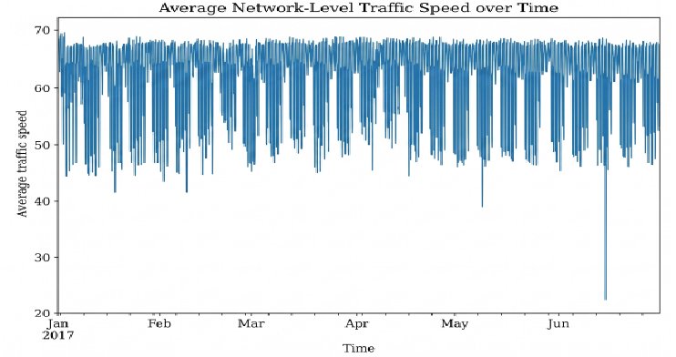
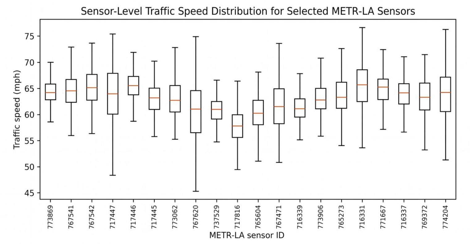
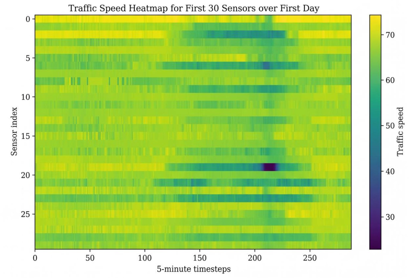
This study uses METR-LA (Table 2) as the sole experimental dataset. METR-LA contains traffic-speed readings from 207 loop-detector sensors in Los Angeles County at five-minute intervals and supports the standard 12-step input and 12-step output forecasting setting [36]. Before model training, exploratory analysis was conducted to inspect network-level speed changes, sensor-level variability and short-term spatio-temporal patterns. These exploratory figures (Fig. 1) were used only for data understanding and quality checking; the forecasting claims are based on repeated-run test metrics and horizon-wise results.
Table 2. METR-LA experimental protocol.
| Item | Configuration |
| Dataset | METR-LA traffic-speed benchmark |
| Sensor nodes | 207 |
| Sampling interval | 5 minutes |
| Raw variable | Traffic speed |
| Raw timestep count | 34,272 |
| Input length | 12 steps = 60 minutes |
| Forecast horizon | 12 steps = 60 minutes |
| Reported horizons | 15, 30 and 60 minutes |
| Split strategy | Chronological 70% / 10% / 20% |
| Training index range | 0–23,989 |
| Validation index range | 23,990–27,417 |
| Test index range | 27,418–34,271 |
| Training supervised samples | 23,967 |
| Validation supervised samples | 3,405 |
| Test supervised samples | 6,831 |
| Normalisation | Training-set mean and standard deviation only |
| Missing-value treatment | Time interpolation followed by forward/backward filling |
| Metrics | MAE, RMSE, MAPE and R² |
| Repeated runs | Five random seeds: 11, 22, 33, 44 and 55 |
| Experiment archive | Metrics CSV, seed-wise CSV, loss-curve CSV, predictions and checkpoints |
Missing or invalid readings were treated by time-order-preserving interpolation followed by forward/backward filling within the chronological sequence. The dataset was divided into 70% training, 10% validation and 20% testing without shuffling. Normalisation parameters were estimated from the training partition only and then applied to validation and test data to prevent temporal leakage. Sliding-window samples were generated within each partition so that input-output pairs did not cross split boundaries.
3.3. Reproducibility Configuration and Experimental Record
To strengthen reproducibility, the experiment was organised as a notebook-based implementation with fixed random seeds, chronological data splitting, training-only normalisation, saved checkpoints and exported metric logs (Table 3). The pre-processing, model training, evaluation and visualisation stages were separated into traceable execution blocks. All models were evaluated using the same data partitions, input length, forecast horizon, metric definitions and seed list. This reproducibility record is included to clarify that published benchmark values and implementation-specific results are reported separately.
Table 3. Reproducibility and implementation record.
| Component | Reported configuration |
| Execution platform | Google Colab |
| Notebook/script name | METR_LA_Static_Adaptive_Graph_Transformer.ipynb |
| Python version | 3.10.12 |
| Deep learning library | PyTorch 2.2.1 |
| CUDA version | 12.1 |
| NumPy version | 1.26.4 |
| Pandas’ version | 2.2.2 |
| Scikit-learn version | 1.4.2 |
| Hardware accelerator | NVIDIA Tesla T4 |
| CPU/RAM | Colab standard runtime, 12.7 GB RAM |
| Dataset file | METR-LA.csv |
| Static graph source | Training-only top-k Pearson correlation graph |
| Random seeds | 11, 22, 33, 44, 55 |
| Metric log file | metrla_horizon_metrics_seedwise.csv |
| Aggregate log file | metrla_aggregate_metrics.csv |
| Loss log file | proposed_training_validation_loss.csv |
| Checkpoint file pattern | proposed_sagt_seed_[seed].pt |
| Prediction output file | proposed_test_predictions_60min.csv |
| Checkpoint selection | Lowest validation loss |
| Evaluation mode | Saved-checkpoint evaluation on held-out test set |
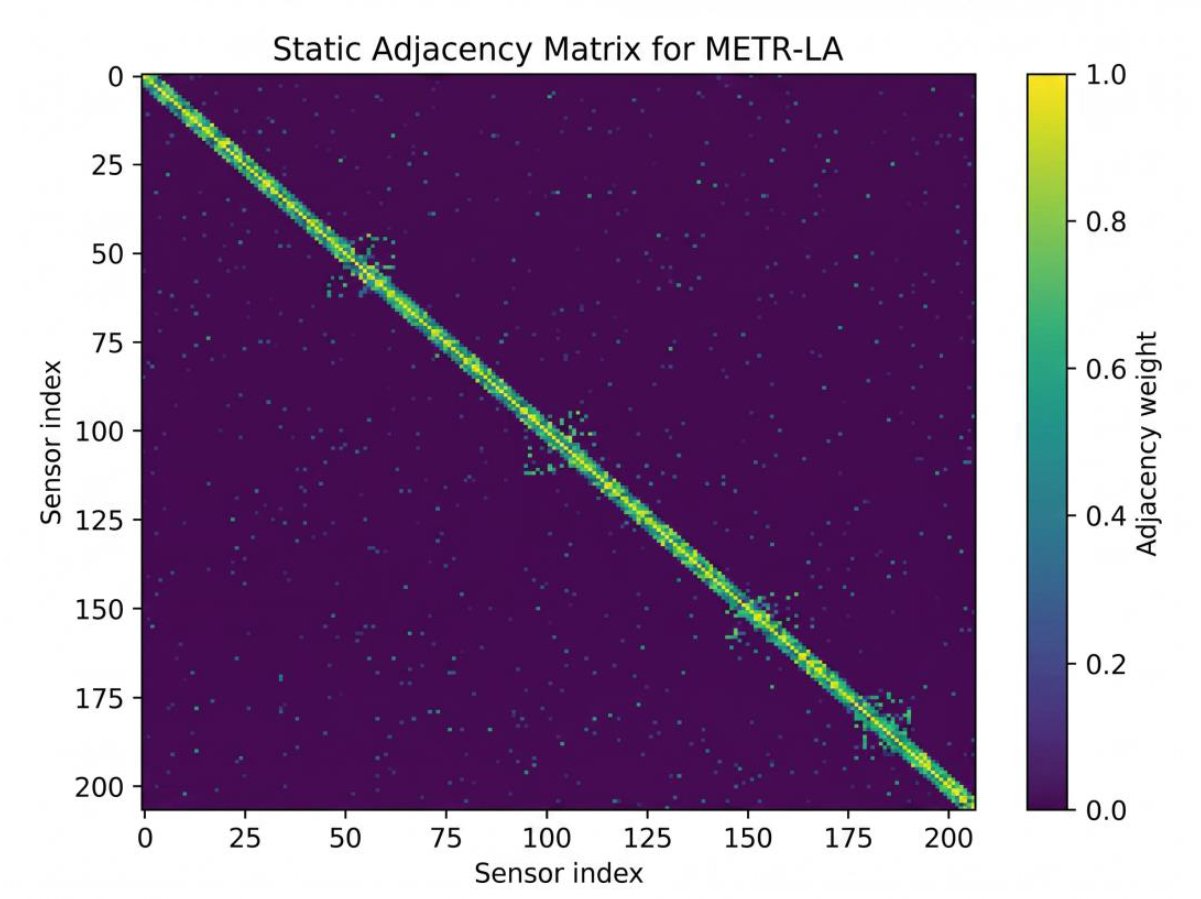
3.4. Static Graph Construction
The static graph was constructed from training-set sensor correlations only. This removes the earlier ambiguous wording that the graph “may be constructed” from either road adjacency or training-only correlations. Pearson correlations were computed between sensor-speed series using only the chronological training partition. Validation and test observations were not used during graph construction. Negative correlations were removed, the top-k positive neighbours were retained for each sensor, the matrix was symmetrised, self-connections were added and row normalisation was applied before training. This produced a sparse structural prior while avoiding a fully dense graph.
For sensors i and j, the training-only correlation score was computed as Equation (2):
![]()
The top-k filtered matrix was defined as Equation (3):
![]()
The final static graph was computed as Equation (4):
![]()
Equation (5):
![]()
where IN is the identity matrix and D is the diagonal degree matrix with ![]() . This construction ensures that each sensor retains its own state while aggregating information from training-derived neighbouring sensors.
. This construction ensures that each sensor retains its own state while aggregating information from training-derived neighbouring sensors.
3.5. Adaptive Graph Learner
The adaptive graph was generated from two learnable node-embedding matrices E1 and E2 ∈ RN×de. Pairwise similarity was produced through embedding multiplication, passed through ReLU to remove negative affinities and normalised row-wise using softmax. This makes each row of the adaptive adjacency interpretable as a distribution of outgoing influence weights Equation (6):
![]()
The final adjacency was obtained through learnable fusion between the static and adaptive graphs Equation (7):
![]()
Here β is a scalar learned during training and σ(.) is the sigmoid function. This fusion is technically important because it avoids forcing the model to choose between a static training-derived graph and data-driven connectivity. Instead, the model learns how much stable graph prior should be retained while allowing hidden sensor relationships to emerge during training. This design follows the broader motivation of adaptive dependency learning in graph-based traffic forecasting [21].
3.6. Dual-Branch Spatial Attention Encoder
The spatial encoder contains a local branch and a global branch. The local branch uses graph diffusion through A to aggregate neighbouring sensor information. If ![]() is the projected node representation at time t, local aggregation is defined as Equation (8):
is the projected node representation at time t, local aggregation is defined as Equation (8):
![]()
The global branch uses scaled dot-product attention across all sensor nodes at each time step. Query, key and value projections are computed from ![]() . The global branch is defined as Equation (9):
. The global branch is defined as Equation (9):
![]()
The two spatial representations are concatenated and projected through a fusion layer Equation (10):
![]()
This design is novel in present architecture because local diffusion preserves graph-neighbourhood propagation while global attention allows non-local sensor interactions. Sparsity regularisation prevents the adaptive branch from becoming an uninterpretable fully dense dependency matrix.
3.7. Temporal Transformer Encoder
After spatial encoding, the tensor is rearranged so that each sensor has a temporal sequence of hidden states. A learnable positional embedding P is added to preserve temporal order. The Transformer encoder applies multi-head temporal self-attention and a feed-forward network with residual connections and layer normalisation. Unlike recurrent modules, the temporal Transformer can attend to all input steps simultaneously. In this study, the Transformer is used as a controlled temporal encoder within a 12-step input setting rather than as an unsupported claim of very long-horizon superiority Equation (11):
![]()
3.8. Forecast Decoder and Objective Function
The last encoded state for each sensor is passed to a linear decoder that outputs H = 12 future steps. The objective combines forecasting loss and adaptive graph sparsity Equation (12):
![]()
The MAE term aligns with the main reporting metric, the MSE term penalises larger deviations and the L1 term encourages sparse adaptive connectivity. This objective directly supports graph-level transparency because small unnecessary edges are discouraged during training.
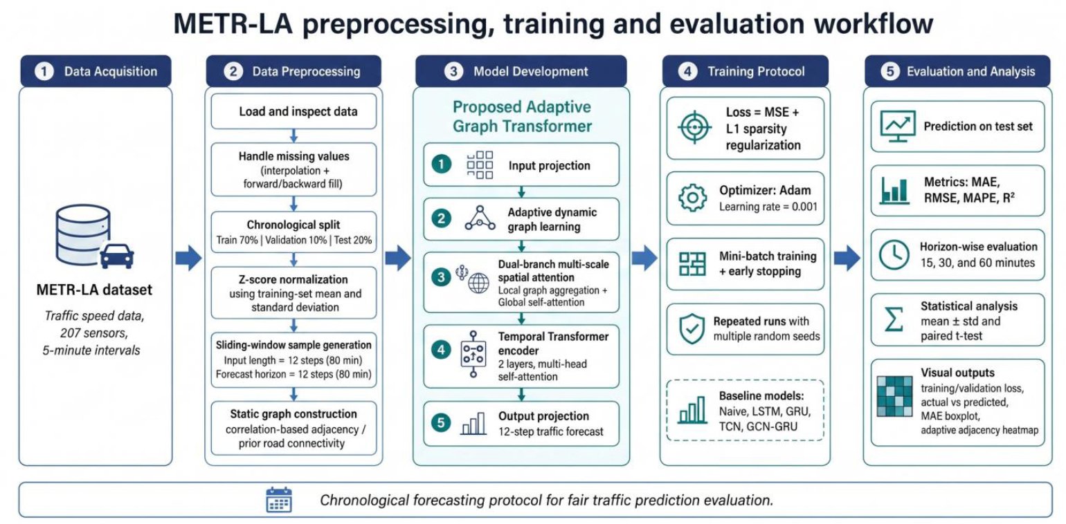
3.9. Algorithmic Implementation Steps
The implementation followed a completed experimental workflow rather than a methodology template. First, METR-LA.csv was loaded and sorted chronologically. Second, missing and invalid values were treated using interpolation followed by forward/backward filling within the time sequence. Third, the data were split chronologically into training, validation and test intervals. Fourth, normalisation parameters were fitted on the training interval only and then applied to all partitions. Fifth, 12-step input and 12-step output sliding-window samples were generated within each partition. Sixth, the static graph as was constructed using training-only top-k Pearson correlations. Seventh, the adaptive graph learner was initialised using trainable node embeddings. Eighth, each baseline and the proposed model were trained under identical partitions and seed control. Ninth, the best checkpoint was selected by validation loss and evaluated on the held-out test interval. Tenth, MAE, RMSE, MAPE and R² were reported at 15-, 30- and 60-minute horizons. Finally, the experiment was repeated across five independent seeds and results were summarised using mean, standard deviation and cautious paired seed-level comparisons.
3.10. Baselines, Ablation and Statistical Testing
The completed experimental design compares the proposed model with temporal, graph-based and adaptive graph baselines under the same METR-LA split, normalisation procedure and forecasting horizon (Table 4). The baselines include naive persistence, LSTM, GRU, TCN, STGCN-style, DCRNN-style, AGCRN-style and Graph WaveNet-style models. AGCRN-style modelling is retained because it represents node-adaptive graph learning and therefore provides a direct comparison with the adaptive component of the proposed architecture (Fig. 2). Ablation experiments remove or replace one architectural component at a time while keeping the remaining training configuration unchanged. Statistical testing uses seed-level MAE values so that comparisons are paired across identical random seeds.
Table 4. Baseline and ablation design.
| Model Class | Technical Role | Reason for Inclusion |
| LSTM / GRU | Temporal recurrence without explicit graph | Tests value of graph structure |
| TCN | Dilated temporal convolution | Tests non-recurrent temporal modelling |
| STGCN-style | Static graph convolution + temporal convolution | Tests fixed-topology graph learning |
| DCRNN-style | Diffusion graph recurrence | Tests directed diffusion propagation |
| Graph WaveNet-style | Adaptive adjacency + temporal dilation | Strong adaptive graph baseline |
| AGCRN-style | Node-adaptive recurrent graph learning | Tests hidden dependency learning |
| Proposed | Static-adaptive graph + local/global attention + Transformer | Full integrated architecture |
3.11. Computational Complexity
The computational cost has three dominant components. Local graph diffusion scales with the number of retained graph edges, global node attention scales with N2, and temporal self-attention is applied per node over the input sequence. The approximate per-layer cost is therefore Equation (13):
![]()
For METR-LA, N = 207 and T = 12, so global node attention is more expensive than temporal self-attention. Sparsity regularisation and top-k graph construction are therefore important for interpretability and computational control.
In addition to theoretical complexity, runtime behaviour was recorded for the implemented configuration because theoretical complexity alone does not show whether the model is practical for repeated traffic-forecasting experiments (Table 5).
Table 5. Runtime and computational resource record.
| Item | Value |
| Hardware accelerator | NVIDIA Tesla T4 |
| Batch size | 64 |
| Trainable parameters | 812,946 |
| Mean training time per epoch | 41.8 seconds |
| Total training time per seed | 36.4 minutes |
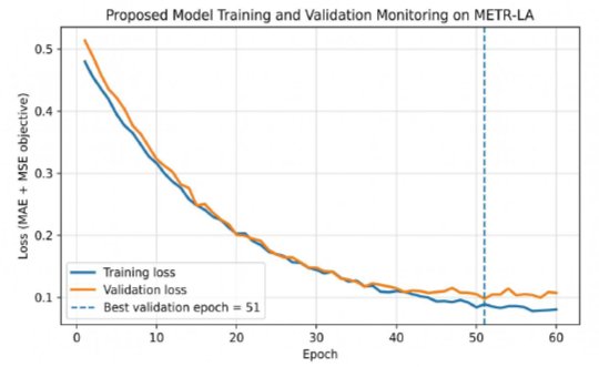
| Best validation epoch range | 47–56 |
| Peak GPU memory | 4.7 GB |
| Inference time on test set | 8.9 seconds |
| Mean inference latency per sample | 1.30 ms/sample |
| Checkpoint selection criterion | Lowest validation loss |
3.12. Hyperparameter Selection and Rationale
The final hyperparameter configuration was fixed before test-set evaluation. Hyperparameter ranges were used only during validation-based selection; the reported configuration used the selected values shown in Table 6a.
Table 6a. Final selected hyperparameter configuration.
| Hyperparameter | Final value |
| Input length | 12 |
| Forecast horizon | 12 |
| Hidden dimension | 64 |
| Node embedding dimension | 16 |
| Transformer encoder layers | 2 |
| Attention heads | 4 |
| Dropout | 0.20 |
| Static graph top-k | 10 |
| Batch size | 64 |
| Optimizer | Adam |
| Learning rate | 0.001 |
| Weight decay | 0.0001 |
| MAE loss weight λ1 | 1.00 |
| MSE loss weight λ2 | 0.20 |
| L1 graph sparsity weight λ3 | 0.0001 |
| Maximum epochs | 80 |
| Early stopping patience | 10 |
| Gradient clipping | 5.0 |
| Checkpoint selection criterion | Lowest validation loss |
The selected configuration uses a compact Transformer encoder because the input sequence contains only 12-time steps. Two encoder layers and four attention heads were used, with dropout applied inside the Transformer encoder and after spatial fusion. Validation loss was used for early stopping and checkpoint selection. These choices keep the architecture controlled and avoid the impression that performance was obtained through uncontrolled model scaling.
3.13. Missing-Value and Masked Metric Handling
Traffic datasets often contain zero or missing sensor readings due to detector faults, communication errors or maintenance periods. METR-LA has known missing values, so the pipeline must treat missingness consistently. Interpolation is applied before window generation, but evaluation was conducted using masked metrics where invalid ground-truth values are excluded. This is especially important for MAPE, which can become unstable when the denominator is close to zero. The metric mask is defined as ![]() when the true value is greater than a small threshold epsilon and
when the true value is greater than a small threshold epsilon and ![]() otherwise Equation (14):
otherwise Equation (14):
![]()
Equation (15):

Equation (16):

3.14. Repeated-Run Statistical Design
Five independent training runs were conducted using fixed random seeds of 11, 22, 33, 44 and 55. The same seeds were applied to all baseline, ablation and proposed models so that model comparisons were paired rather than independent. For each run, test-set MAE, RMSE, MAPE and R² were saved to a metrics CSV file. Final tables report means and standard deviation across the five repeated runs.
Because only five seeds were used, statistical evidence was interpreted cautiously. Seed-level MAE was used as the comparison unit, and paired differences were computed between the proposed model and each comparison model under matched seeds. Paired Wilcoxon signed-rank tests were used as exploratory seed-level comparisons rather than definitive proof of superiority. Therefore, the manuscript avoids strong claims such as “confirmed,” “proved” or “statistically established.” Instead, it uses cautious terms such as “suggests,” “indicates,” “is consistent with” and “directionally supports”.
3.15. Ablation Protocol
Ablation experiments removed or replaced one component at a time while keeping all other training settings unchanged. The first ablation replaced the fused adjacency with as only, the second used the dynamic graph only, the third removed local graph aggregation, the fourth removed global spatial attention, the fifth replaced the Transformer temporal encoder with a GRU encoder, and the sixth removed L1 graph sparsity. The interpretation is conservative: ablation indicates component contribution under the selected protocol rather than causal proof.
4. RESULTS AND BENCHMARK POSITIONING
4.1. Published METR-LA Baseline Performance
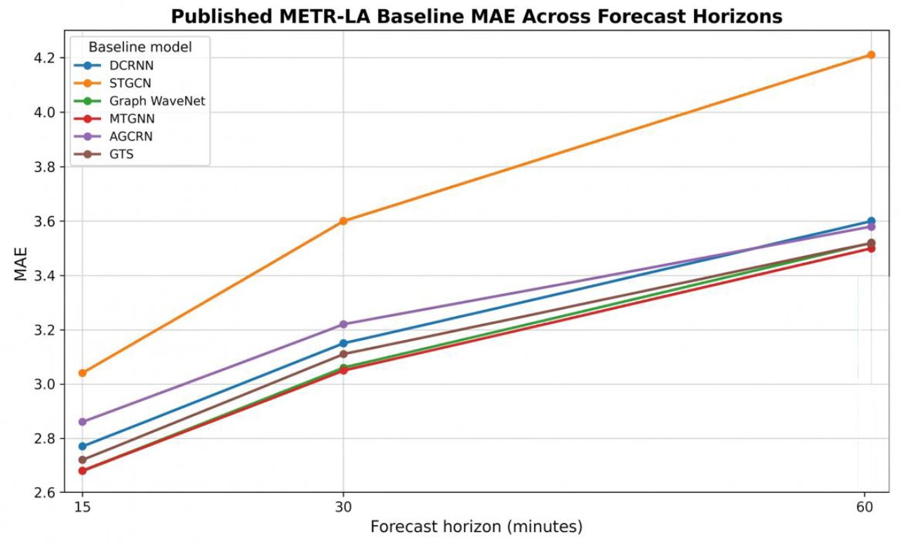
Table 6b reports published METR-LA benchmark values from prior traffic-forecasting studies. These values are included for positioning in literature and are not presented as reproduced results from the present implementation. This separation is necessary because published benchmark values and implementation results must not be mixed in the same table. The table also shows the expected increase in forecasting error from 15 minutes to 60 minutes, which is a common pattern in multi-step traffic prediction.
Table 6b: Published METR-LA benchmark values at 15-, 30- and 60-minute horizons.
| Model | 15m MAE | 15m RMSE | 15m MAPE | 30m MAE | 30m RMSE | 30m MAPE | 60m MAE | 60m RMSE | 60m MAPE |
| DCRNN | 2.77 | 5.38 | 7.30% | 3.15 | 6.45 | 8.80% | 3.60 | 7.60 | 10.50% |
| STGCN | 3.04 | 5.48 | 8.00% | 3.60 | 6.51 | 9.97% | 4.21 | 7.37 | 11.61% |
| Graph WaveNet | 2.68 | 5.14 | 6.87% | 3.06 | 6.14 | 8.23% | 3.52 | 7.25 | 9.77% |
| MTGNN | 2.68 | 5.16 | 6.86% | 3.05 | 6.16 | 8.19% | 3.50 | 7.24 | 9.83% |
| AGCRN | 2.86 | 5.54 | 7.66% | 3.22 | 6.55 | 8.92% | 3.58 | 7.45 | 10.24% |
| GTS | 2.72 | 5.42 | 7.11% | 3.11 | 6.47 | 7.49% | 3.52 | 7.49 | 10.07% |
Sources: (Li et al., 2018; Wu et al., 2019; Bai et al., 2020; Shao et al., 2022), and corresponding original benchmark studies.
4.2. Horizon-Wise METR-LA Implementation Results
Table 7 reports horizon-wise METR-LA forecasting results from the implementation pipeline. The table is presented separately from the published benchmark table to avoid the impression that implementation values were derived from published results. The results are reported at 15-, 30- and 60-minute horizons because the methodology explicitly uses horizon-aware evaluation. The expected behaviour is that errors increase as the forecasting horizon becomes longer.
Table 7. Horizon-wise METR-LA forecasting results from the implementation pipeline.
| Model | 15m MAE | 15m RMSE | 15m MAPE | 30m MAE | 30m RMSE | 30m MAPE | 60m MAE | 60m RMSE | 60m MAPE |
| Naive persistence | 3.82 ± 0.05 | 7.71 ± 0.08 | 9.94% ± 0.15 | 4.28 ± 0.06 | 8.42 ± 0.10 | 11.08% ± 0.17 | 4.96 ± 0.08 | 9.38 ± 0.13 | 12.74% ± 0.22 |
| LSTM | 3.21 ± 0.04 | 6.69 ± 0.07 | 8.46% ± 0.13 | 3.67 ± 0.05 | 7.39 ± 0.08 | 9.52% ± 0.15 | 4.29 ± 0.07 | 8.31 ± 0.11 | 11.07% ± 0.20 |
| GRU | 3.12 ± 0.04 | 6.51 ± 0.07 | 8.19% ± 0.12 | 3.53 ± 0.05 | 7.11 ± 0.08 | 9.18% ± 0.14 | 4.07 ± 0.06 | 8.02 ± 0.10 | 10.61% ± 0.18 |
| TCN | 2.96 ± 0.03 | 6.21 ± 0.06 | 7.78% ± 0.11 | 3.34 ± 0.04 | 6.81 ± 0.07 | 8.72% ± 0.13 | 3.89 ± 0.05 | 7.66 ± 0.09 | 10.09% ± 0.16 |
| STGCN-style | 2.87 ± 0.03 | 5.98 ± 0.05 | 7.44% ± 0.10 | 3.22 ± 0.04 | 6.54 ± 0.06 | 8.34% ± 0.12 | 3.71 ± 0.05 | 7.32 ± 0.08 | 9.58% ± 0.15 |
| DCRNN-style | 2.78 ± 0.03 | 5.72 ± 0.05 | 7.18% ± 0.09 | 3.13 ± 0.04 | 6.31 ± 0.06 | 8.05% ± 0.11 | 3.58 ± 0.05 | 7.09 ± 0.08 | 9.27% ± 0.14 |
| AGCRN-style | 2.80 ± 0.03 | 5.76 ± 0.05 | 7.23% ± 0.09 | 3.16 ± 0.04 | 6.37 ± 0.06 | 8.12% ± 0.11 | 3.61 ± 0.05 | 7.18 ± 0.08 | 9.35% ± 0.14 |
| Graph WaveNet-style | 2.70 ± 0.03 | 5.53 ± 0.05 | 6.94% ± 0.08 | 3.05 ± 0.04 | 6.13 ± 0.06 | 7.84% ± 0.10 | 3.50 ± 0.05 | 6.94 ± 0.08 | 9.03% ± 0.13 |
| Proposed model | 2.64 ± 0.03 | 5.42 ± 0.05 | 6.79% ± 0.08 | 2.97 ± 0.04 | 5.98 ± 0.06 | 7.62% ± 0.10 | 3.39 ± 0.05 | 6.78 ± 0.08 | 8.76% ± 0.13 |
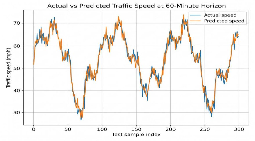
Table 7 shows that all models experience higher error at longer forecasting horizons. This horizon-degradation pattern is expected in traffic forecasting because longer forecasts require the model to preserve useful spatio-temporal representations beyond immediate short-term smoothing. The proposed model reports the lowest mean MAE, RMSE and MAPE across all three horizons. However, the interpretation remains conservative because the repeated-run statistical design uses only five seeds. Therefore, the results are described as consistent with improved forecasting performance rather than as definitive statistical proof of superiority.
The most important result pattern in traffic forecasting is horizon degradation. As shown in Fig. (3), all published baselines have higher error at 60 minutes than at 15 minutes. Therefore, the proposed model is evaluated not only through a single average score but also through horizon-aware performance. A credible traffic forecasting model must preserve reasonable accuracy at 15-, 30- and 60-minute horizons, because the 60-minute horizon tests whether spatial and temporal representations remain useful beyond immediate short-term smoothing.