

- ABSTRACT:
- 1. INTRODUCTION
- 2. LITERATURE REVIEW
- 3. METHODOLOGY
- 3.1. System Architecture
- 3.2. Dataset Description
- 3.3. Feature Engineering
- 3.4. Model Architecture
- 3.5. Evaluation Metrics
- 3.6. Cross-Validation, Dependence Structure, and Confidence-Interval Reporting
- 3.7. Component-Level Numerical Ablation Design
- 3.8. Measured RAN Testbed Evaluation Design
- 3.9. Longer DQN Training, Baselines, and Integration Interface
- 4. RESULTS AND DISCUSSION
- 4.1. Classification Model Performance Analysis
- 4.2. Feature Impact Analysis Using SHAP
- 4.3. Exploratory Data Insights
- 4.4. Preliminary 4,680-Step Simulation DQN Diagnostics
- 4.5. Comparative Interpretation and Implications
- 4.6. Numerical Component-Ablation Results
- 4.7. Measured RAN Next-Step CQI Prediction Results
- 4.8. Principal 50,000-Step DQN and Offline Measured-Trace Baseline Results
- LIMITATIONS
- CONCLUSION
- LIST OF ABBREVIATIONS
- AUTHOR'S CONTRIBUTION
- ETHICAL APPROVAL & INFORMED CONSENT
- AVAILABILITY OF DATA AND MATERIALS
- FUNDING
- CONFLICT OF INTEREST
- ACKNOWLEDGEMENTS
- DECLARATION OF AI
- REFERENCES
Article ID: PD2601202008
Views: 51Interpretable Quality-of-Service and Channel-Quality-Indicator State Prediction and Offline Allocation Scoring with Extreme Gradient Boosting and Deep Q-Networks: Simulation and Measured Radio-Access-Network Trace Evidence
⬇ Downloads: 3
1Department of Computer Science and Engineering, Biju Patnaik University of Technology (BPUT), Odisha, India
Revised: 03 October, 2026
ABSTRACT:
Introduction: Fifth-generation (5G) networks require adaptable and explainable mechanisms for quality-of-service (QoS) and channel-quality-indicator (CQI) state prediction and resource-allocation analysis.
Methodology: This study evaluates a two-stage Extreme Gradient Boosting (XGBoost)-Deep Q-Network (DQN) decision-support framework in which supervised prediction and allocation-policy scoring are deliberately separated.
Results: In the legacy simulation-derived branch, XGBoost achieved accuracy and macro F1 of 0.87 on an archived 79-window held-out subset. Because lagged-window sequence membership and the exact 527-window construction are not recoverable, this result and the historical random five-fold values are reported descriptively rather than as temporal-generalisation evidence. Measured validation used 27,720 observations from the EURECOM ElasticMon radio access network (RAN) testbed and a study-defined one-step-ahead CQI target. XGBoost achieved pooled accuracy 0.960 and macro F1 0.937, whereas random forest achieved 0.971 and 0.949; XGBoost mean held-out-partition macro F1 was 0.685 ± 0.307, demonstrating substantial partition heterogeneity. For offline allocation scoring, five 50,000-step DQN runs were evaluated on two held-out measured traces. Integrated XGBoost-DQN obtained a mean score of 1.092 ± 0.465 versus 1.062 ± 0.470 for DQN-only; the paired mean difference of 0.030 had a bootstrap 95% confidence interval (CI) of -0.016 to 0.080. Mean over-allocation was 0.222 versus 0.289, while measured-CQI shortfall remained 20.4% for every policy because actions did not alter recorded trace outcomes.
Conclusion: The evidence supports interpretable next-step state prediction and comparative offline allocation scoring, not causal resource control or commercial-network efficiency.
Keywords: 5G network slicing, XGBoost, Deep Q-Network, SHapley Additive exPlanations (SHAP), offline allocation scoring, measured RAN testbed data, CQI classification, trace-driven evaluation.
1. INTRODUCTION
Fifth-generation (5G) mobile networks represent a major advance in wireless communications, offering high data capacity, low latency and connectivity for large numbers of devices [1]. Enabling technologies such as massive multiple-input multiple-output (MIMO), millimetre-wave (mmWave) communication and network slicing support scalable, service-specific performance guarantees [2]. Massive MIMO increases spectral efficiency through spatial multiplexing, while mmWave bands provide wider bandwidths but introduce propagation challenges that require intelligent beamforming and dynamic link management [3]. Network slicing further divides the physical infrastructure into logical slices optimised for enhanced mobile broadband (eMBB), ultra-reliable low-latency communications (URLLC) and massive machine-type communications (mMTC) [4].
Artificial intelligence (AI) and machine learning (ML) are increasingly used to support automation and optimisation in 5G networks. Data-driven systems can adapt decisions to near-real-time observations rather than relying only on static policies. AI/ML techniques are applied throughout the 5G stack, including channel estimation and modulation classification at the physical layer, and resource scheduling, mobility prediction and energy-efficient handover at higher layers [5]. Adaptive capability becomes more important as networks must support heterogeneous devices, changing service demands and time-varying traffic under limited resources [6].
Although 5G technology continues to standardise, traditional rule-based and heuristic optimisation methods can struggle to adapt to rapidly changing network conditions [7]. Such methods typically depend on predetermined thresholds or fixed policies and are therefore only weakly context-sensitive. For example, a policy that performs adequately under moderate traffic may become inefficient during concentrated or rapidly changing demand [8]. Likewise, legacy approaches may not adequately distinguish quality-of-service requirements between applications such as video streaming and safety-critical communications [9].
Limited adaptive learning can therefore affect load balancing, spectrum allocation and network slicing [10]. In real-time slice orchestration, agents must respond to environmental feedback [11]; otherwise, operators may experience higher operating costs, reduced quality of service and avoidable resource waste. Diversity in user devices, mobility patterns and service-level agreements (SLAs) consequently motivates data-driven optimisation techniques that can be evaluated under varied network conditions [12].
While research on AI/ML for 5G has grown significantly, much of the reported work remains simulation-based and/or relies on a single model. Although controlled simulation is economical and reproducible, it cannot fully capture noise, outliers, varying traffic distributions, and operational constraints [13, 14]. Therefore, results from a simulation-derived dataset should be viewed as evidence of concept, not as direct evidence of real-world performance.
Recent work shows that prediction and reinforcement learning (RL) can both contribute to 5G resource management, but they answer different questions. Supervised models estimate states or outcomes, whereas an RL agent selects sequential actions under a defined environment and reward function [15, 16]. Current online-control research includes actor-critic and multi-agent deep reinforcement learning (DRL) formulations, as discussed in Section 2.4. The present study therefore treats prediction and decision/scoring as separate evidence layers and tests whether XGBoost class probabilities add information to a DQN state under a common action space, rather than assuming that predictive accuracy establishes control effectiveness.
A further research gap concerns the limited integration of network slicing and cross-layer optimisation within AI-based decision frameworks. Many studies focus on a single objective, such as throughput, delay or energy efficiency, without jointly representing priorities and dependencies across radio-access and core-network functions. This narrower modelling scope can be restrictive in operational settings where competing key performance indicators (KPIs) and service requirements must be balanced.
To address this gap within a deliberately bounded experimental framework, the study uses two linked components. XGBoost performs data-defined state prediction, and SHapley Additive exPlanations (SHAP) are used to interpret the fitted prediction function. A single-agent DQN then selects one of three discrete allocation multipliers. In the integrated configuration, the three XGBoost class probabilities are appended to the DQN state; XGBoost-only and DQN-only configurations provide component comparators. The simulation-derived and measured EURECOM experiments are reported as distinct evidence tiers because they use different targets, environments and interpretations.
The study aims to (i) evaluate XGBoost for supervised QoS-state classification in the original simulation-derived experiment; (ii) interpret the classifier with SHAP and test sensitivity to alternative QoS-label definitions; (iii) quantify the incremental value of XGBoost probabilities through 20 paired algorithm reruns within one simulated environment; and (iv) evaluate next-step CQI-class prediction and comparative allocation scoring on measured EURECOM RAN traces using held-out analysis partitions and explicit offline baselines. The study does not claim causal resource-allocation effects, commercial operator-network validation or production-deployment readiness.
The key innovation is the explicit probability-vector interface from interpretable XGBoost state prediction to a DQN, evaluated by component ablation while keeping measured-trace prediction separate from offline allocation scoring.
The principal contribution is an evidence-bounded prediction-to-scoring interface rather than a new autonomous 5G controller. It combines interpretable supervised state probabilities with a DQN state, tests that interface through component ablation, and then separates simulation evidence from measured RAN evidence. The 4,680-step simulation output is treated only as a preliminary diagnostic; the principal measured-trace DQN comparison uses a 50,000-step budget and five reported seeds. Measured-trace allocation results are interpreted as counterfactual offline scores because the chosen action cannot change the next recorded CQI.
2. LITERATURE REVIEW
2.1. Traditional 5G Optimisation Techniques
Traditional 5G optimisation has often relied on heuristic and rule-based systems, including pre-set decision rules, engineering-defined thresholds and fixed policies. Although these methods are simple and transparent, they may be insufficient for nonlinear, time-varying environments [17–19]. Fixed resource-allocation policies can become inefficient when demand changes unexpectedly.
Traditional telecommunications management can also be highly centralised. Network operations centres and central control functions simplify supervision but can introduce latency or bottlenecks when near-real-time decisions are required [20]. Distributed, virtualised and open-network architectures, including network function virtualisation (NFV), software-defined networking (SDN) and Open Radio Access Network (O-RAN), can move intelligence closer to the radio edge and support faster local responses [21]. However, distributed rule-based systems without adaptive AI/ML can still struggle with rapidly changing traffic and radio conditions.
2.2. AI and ML in Telecom Networks
The use of machine learning and artificial intelligence is growing to enable adaptive and predictive features in 5G and beyond-5G systems [18, 19]. Besides classification and anomaly detection, classical approaches like Support Vector Machines and Random Forests are still applicable and can be used for modern telecom analytics like throughput, mobility, handover, resource management and energy efficiency [22]. When choosing models, it is important to consider data structure, decision latency and operational constraints; assumptions of the superiority of one family of models should not be made.
Extreme Gradient Boosting (XGBoost) is a regularised tree-boosting method that can model nonlinear interactions in tabular data and is widely used in predictive modelling [23–25]. In telecommunications applications, tree-boosting models can be used to predict throughput, delay, jitter, channel condition or service-state indicators. In this study, XGBoost is used as a supervised classifier; the resulting associations are predictive rather than causal.
Convolutional neural networks (CNNs) and long short-term memory (LSTM) networks are established deep-learning architectures for spatial and sequential learning, respectively [26, 27]. CNNs are used in signal- and spectrum-related applications, while recurrent networks can model traffic or mobility sequences. For the present proof-of-concept setting, their greater computational and data requirements support the use of a simpler tabular classifier.
Graph neural networks (GNNs) can represent topological dependence among users, base stations and network functions, and broader 5G and sixth-generation (6G) surveys discuss such topology-aware learning directions [28]. Mobility and handover studies likewise show that context and temporal structure matter for radio decisions [29]. Federated learning provides another edge-centric option by reducing centralisation of raw data, although convergence, statistical heterogeneity and communication overhead remain important design constraints.
2.3. Reinforcement Learning (RL)
Reinforcement learning (RL) learns sequential decisions through states, actions and rewards. For discrete actions, Deep Q-Networks (DQN) combine Q-learning with a neural action-value approximator [21]. Deep RL has also been applied to slice-aware resource-management problems [29–31]. In this study, DQN is used as a constrained experimental decision/scoring component rather than as an expert autonomous controller, with only three discrete allocation multipliers.
For continuous actions such as transmission power, policy-gradient and actor-critic methods provide finer control but require careful stability and hyperparameter management. Multi-agent and federated actor-critic approaches have also been proposed for network slicing and multi-RAN resource allocation; representative recent methods are compared in Section 2.4. These approaches target active optimisation in simulated or modeled environments, whereas the measured-trace branch in the present study is intentionally narrower because its recorded radio outcomes are observational and cannot be altered by the evaluated policy.
These advances have not yet produced extensive deployment-quality RL evidence for telecommunications. Simulation and testbed studies remain common because online exploration can be hazardous, convergence can be slow, and policy decisions can be difficult to explain. Sparse or delayed network feedback further complicates learning. These constraints motivate a bounded decision-support design that combines interpretable supervised prediction with a tightly controlled sequential decision component rather than claiming autonomous operation.
2.4. Novelty Positioning
Recent approaches provide useful comparison points. Ejaz et al., [32] formulate end-to-end slicing as an online multi-agent DRL allocation problem in mobile-edge-computing simulations, while Azimi et al., [33] combine federated advantage actor-critic resource allocation with stacked bidirectional long short-term memory (SBiLSTM) prediction in a multi-RAN slicing architecture. These studies emphasise active control and optimisation. By contrast, the present work does not propose a new RL algorithm or claim control superiority; its methodological novelty is the explicit separation and quantitative linking of interpretable supervised state prediction, component-level DQN ablation and measured-trace offline scoring under clearly stated evidence boundaries.
Four design choices distinguish the present framework from a single-model prediction or control study: (1) the full low/medium/high XGBoost probability vector, rather than only a hard predicted class, is appended to the DQN state and tested against a DQN-only comparator; (2) SHAP and three alternative QoS-label schemes are used to expose what drives prediction and how label design changes class-level recall; (3) measured EURECOM telemetry is evaluated using leave-one-analysis-partition-out next-step CQI prediction with logistic-regression, histogram-gradient-boosting and random-forest baselines; and (4) measured-trace policy results are reported as offline allocation scores with fixed recorded outcomes, so predictive evidence is not converted into a causal control claim.
Accordingly, the term framework denotes a decision-support and evaluation pipeline. The 20 paired algorithm reruns can establish consistency only within the single defined simulated environment; they are not independent network replications. The measured-trace branch strengthens evidence by adding held-out RAN telemetry and several predictive/allocation baselines, but its principal DQN comparison covers two held-out traces and the integrated-versus-DQN score interval spans zero. Practical conclusions are therefore limited to proof-of-concept prediction and offline comparative scoring.
3. METHODOLOGY
3.1. System Architecture
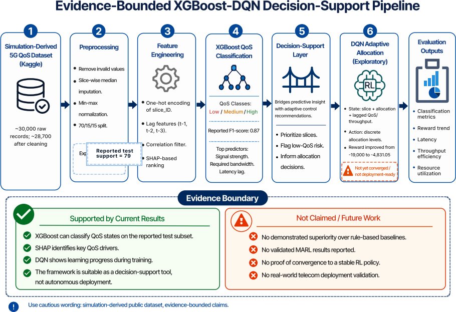
Fig. (1) depicts only the original simulation-derived branch. It shows data cleaning, chronological lag construction, encoding, training-only threshold estimation, XGBoost class-probability generation, DQN integration and SHAP interpretation. The EURECOM next-step CQI validation and the separate 50,000-step trace-driven experiment are reported in Sections 3.8-3.9 and 4.7-4.8 and should not be inferred from the simulation schematic.
Fig. (1). Simulation-Derived XGBoost-DQN Decision-Support pipeline, component flow and evidence boundary.
3.2. Dataset Description
The study uses two data sources with different roles. Reference [34] is the primary public Kaggle 5G QoS/resource-allocation asset. A published analysis of the same asset reports 400 samples with Timestamp, User_ID, Application_Type, Signal_Strength, Latency, Required_Bandwidth, Allocated_Bandwidth and Resource_Allocation fields [35]. The original simulation/QoS experiment in this paper was performed on an archived project derivative that is not identical to the raw Kaggle asset. External measured-data evaluation uses the EURECOM ElasticMon RAN dataset, which contains medium access control (MAC), radio resource control (RRC) and packet data convergence protocol (PDCP) measurements from a FlexRAN/OpenAirInterface testbed [36]. Because the simulation and EURECOM branches use different fields and targets, their results are not treated as interchangeable validation of one label.
The archived project materials describe the simulation-derived working table as approximately 30,000 time-indexed rows containing slice_ID, allocation percentage, QoS_score, throughput, delay/latency, signal strength, required bandwidth, allocated bandwidth and application type.
Within the archived derivative analysis, the recorded preprocessing sequence was removal of physically invalid or incomplete observations, limited within-slice median substitution, min-max scaling of continuous variables, chronological construction of one-, two- and three-step lag features, screening, and selection of a 527-window supervised subset. The archived split was 369 training, 79 validation and 79 held-out windows. However, the exact retention predicates, balancing order, pre/post-balancing class counts, sampling seed, replacement policy, duplicate policy and sequence-level membership were not archived. Because these details cannot be reconstructed reliably, no sampler implementation or class counts are inferred. Table 1 distinguishes documented facts from unavailable provenance, and the 527-window branch is treated as legacy descriptive evidence rather than a leakage-safe temporal benchmark.
Table 1. Provenance, modelling subset, and split reconciliation for the legacy Simulation-Derived branch.
| Dataset-Use Item | Value / Clarification |
| Raw public source | Kaggle 5G QoS/resource-allocation asset [34]: 400 samples and eight source fields, independently described for the same asset in [35]. |
| Archived project derivative | Approximately 30,000 time-indexed rows described in archived project materials; not identical to raw [34]; augmentation/simulation generator not archived. |
| Cleaned derivative / modelling subset | Approximately 28,700 rows recorded after cleaning/feature construction; 527 lagged windows subsequently used for modelling; exact retention/sampler code not archived. |
| Split used | Train 369 / validation 79 / test 79; total support = 527 |
| Selection rule | Exact screening/retention predicates are not archived and cannot be reconstructed without inventing undocumented steps. |
| Balancing order | Not preserved; it cannot be verified whether selection/balancing occurred before or after splitting. |
| Class counts | Not preserved for the 527-window construction stage. |
| Sampling/duplicates | Not preserved; replacement and possible duplicate generation cannot be excluded. |
| Sequence overlap | Not verifiable; neighbouring lagged windows may originate from the same underlying sequence. |
| Interpretation | Legacy descriptive subset only; the random folds and archived held-out subset are not treated as leakage-safe temporal validation or evidence of temporal generalisation. |
To make prediction of the QoS state interpretable, QoS_score was transformed into three supervised-learning classes. Using training-data percentiles, the lowest 20% of QoS_score values were labelled Low, the middle 60% Medium and the highest 20% High. The 20/60/20 scheme separates clearly degraded and high-performing states while retaining a broad middle operating region. To avoid threshold leakage, the P20 and P80 cut-points were estimated from the training subset only and then applied unchanged to the archived validation and held-out subsets.
Three QoS-class construction schemes were compared for threshold sensitivity. In the primary scheme, the bottom 20% of training QoS scores were labelled Low, the middle 60% Medium and the top 20% High. The tertile scheme used the 33.3rd and 66.7th percentiles of the training data to produce approximately equal class intervals. In both cases, thresholds were estimated only from the training subset and applied unchanged to the archived validation and held-out subsets.
A third, SLA-oriented scheme was defined using application-specific latency limits together with bandwidth-fulfilment conditions. The bandwidth-fulfilment ratio was calculated as:
(1)
For the SLA-oriented scheme, let r_L = observed latency / application-specific latency threshold and r_B = allocated bandwidth / required bandwidth. Labels were assigned in a fixed, mutually exclusive order: High if r_L <= 1.00 and r_B >= 1.00; otherwise Medium if r_L <= 1.20 and r_B >= 0.80; otherwise Low. Thus Medium captures only a mild latency overrun (up to 20%) and/or mild bandwidth shortfall (up to 20%) after the High condition has failed, whereas any latency overrun greater than 20% or bandwidth shortfall greater than 20% is Low. This ordered Boolean rule removes overlap between the Medium and Low definitions.
International Telecommunication Union Telecommunication Standardization Sector (ITU-T) Recommendation G.1010 gives preferred one-way delay targets of less than 150 ms for conversational voice and videophone services, less than 200 ms for interactive games, less than 2 seconds for web access, less than 10 seconds for one-way streaming and less than 15 seconds for bulk data transfer. These application-experience targets are distinct from the 4 ms eMBB and 1 ms URLLC radio-interface evaluation requirements specified in International Telecommunication Union Radiocommunication Sector (ITU-R) Recommendation M.2410 under its stated evaluation conditions.
The 50 ms emergency-service threshold in Table 2 is a study-defined conservative operational rule used only for the SLA-oriented sensitivity analysis; it is not presented as a generic standards-mandated emergency-service latency. A 50 ms remote process-control example concerns a different use case and is therefore not used here as evidence for the emergency-service label.
Table 2. Application-specific latency thresholds used in the SLA-Oriented sensitivity scheme.
| Application Category | Latency Threshold | Basis Used in the Study |
| Emergency service | 50 ms | Study-defined conservative 50 ms rule; not standards-mandated |
| Voice call | 150 ms | ITU-T G.1010 preferred conversational-voice target |
| Video call | 150 ms | ITU-T G.1010 preferred videophone target |
| Online gaming | 200 ms | ITU-T G.1010 interactive-game target |
| Web browsing | 2,000 ms | ITU-T G.1010 preferred web-access target |
| Video streaming | 10,000 ms | ITU-T G.1010 one-way streaming target |
| File download | 15,000 ms | ITU-T G.1010 preferred bulk-transfer target |
| IoT temperature monitoring | 1,000 ms | Study-defined non-critical telemetry rule |
The same train/validation/held-out observations, preprocessing, feature set, XGBoost hyperparameters and random seed were retained across the three label schemes. Three performance measures (macro F1, weighted F1 and class-specific recall) were compared descriptively to assess sensitivity to label construction (Section 4.1). No inferential significance test was performed for this comparison; accordingly, the reported differences are interpreted as descriptive sensitivity rather than statistically significant differences.
3.3. Feature Engineering
To improve temporal awareness, systematic feature engineering was applied to the simulation-derived data. slice_ID was one-hot encoded to represent the recorded slice categories (eMBB, URLLC, mMTC and Internet of Things (IoT)) without imposing an artificial ordinal relationship.
Short-term history was represented by one-, two- and three-step lags of throughput and QoS_score within each recorded slice sequence. For a prediction at time t, only values observed at t-1, t-2 and t-3 were eligible; current QoS_score(t), from which the target class was constructed, was not included as a predictor, and no t+1 or later observation entered the feature vector. Lag construction was performed after chronological ordering within each slice. Because adjacent lagged windows share history, random fold assignment can place strongly dependent neighbours in training and validation partitions. Ordinary five-fold cross-validation is therefore retained only as an archival exploratory diagnostic and is not evidence of temporal generalisation. Blocked temporal, forward-chaining or sequence-group validation is methodologically preferred [24], but a faithful rerun of the original 527-window branch cannot be reconstructed because sequence-level retention/sampling provenance was not archived.
Feature screening used correlation analysis, mutual information and SHAP interpretation. Highly collinear predictors (|r| > 0.85) were removed as redundant, mutual-information scores were used to assess dependence with the target class, and SHAP values were used to rank contributions to the fitted XGBoost prediction function. These rankings are model-based predictive associations, not causal effects.
3.4. Model Architecture
The system contains two interdependent but distinct tasks: supervised state prediction and allocation-policy evaluation. XGBoost predicts a three-class state and SHAP interprets the fitted prediction function. In the integrated configuration, the predicted low/medium/high probability vector is concatenated with the normalised network state before DQN action selection. The simulation target is QoS_score, whereas the measured external prediction target is a study-defined next-step CQI class. Classification metrics, RL rewards and offline allocation scores therefore measure different quantities and are not presented as interchangeable evidence.
In the simulation branch, XGBoost used the multiclass probability objective multi:softprob with num_class = 3, so each engineered feature vector produced probabilities for the Low, Medium and High classes. In the integrated configuration, this three-component probability vector was appended to the simulated network state before DQN action selection. The simulated environment then applied the selected allocation action, updated its simulated latency, QoS, bandwidth mismatch and SLA status, and returned reward and next state. This action-responsive simulation must not be conflated with the later EURECOM trace-driven branch, where recorded radio outcomes are fixed and cannot be causally changed by the evaluated action.
Multi-agent reinforcement learning (MARL) is discussed only as related and future work. No MARL experiment or MARL performance metric is reported in this study; the completed allocation experiments use a single-agent DQN. This scope restriction avoids attributing untested multi-agent capability to the proposed framework.
For the simulation DQN, the reward was defined to balance QoS improvement, latency reduction and bandwidth-allocation efficiency. The reward at decision step t was:
(2)
The terms in Equation (2) are defined as follows:
In Equation (2), R_t is reward at time t, ΔQoS_t is the change in QoS score from the previous simulated step, L_t is normalised latency, B_t^alloc is allocated bandwidth, B_t^req is required bandwidth, and V_t is a binary SLA-violation indicator. The absolute bandwidth-mismatch term penalizes both under- and over-allocation. The coefficients were α = 1.00, β = 0.40, γ = 0.30 and δ = 1.00. Continuous reward components were min-max normalised so that scale differences did not dominate the score.
Table 3 separates documented settings from implementation fields that are no longer recoverable. XGBoost used multi:softprob with num_class = 3 and mlogloss, making the three class probabilities explicit for subsequent DQN integration. Recorded DQN settings include learning rate 0.0001, discount factor 0.99, replay buffer 10,000, batch size 32, exploration from 1.00 to 0.05 over a 0.20 exploration fraction, a 250-step target-update interval, three absolute allocation multipliers (0.75/1.00/1.25), a 48-unit hidden layer, five principal seeds (11, 22, 33, 44, 55), and a 50,000-environment-step principal budget. Activation function, optimiser, gradient clipping, replay warm-up, training/update frequency, hard/soft target-update coefficient, terminal-state handling, exact principal episode count, complete RNG propagation, checkpoint initialisation/reuse, package versions and hardware identifier were not archived. Exact bitwise reproduction of the historical DQN training is therefore not claimed.
Table 3. Documented XGBoost and DQN configuration, fixed-budget settings, and unarchived fields.
| Model | Hyperparameter | Value |
| XGBoost | Objective | multi:softprob (num_class = 3) |
| XGBoost | Evaluation metric | mlogloss |
| XGBoost | Number of estimators | 300 |
| XGBoost | Maximum tree depth | 4 |
| XGBoost | Learning rate | 0.05 |
| XGBoost | Subsample ratio | 0.80 |
| XGBoost | Column sample by tree | 0.80 |
| XGBoost | Minimum child weight | 1 |
| XGBoost | Gamma regularization | 0 |
| XGBoost | Random seed | 42 |
| DQN | Policy | Multilayer perceptron (MLP) policy |
| DQN | Learning rate | 0.0001 |
| DQN | Discount factor | 0.99 |
| DQN | Replay buffer size | 10,000 |
| DQN | Batch size | 32 |
| DQN | Initial exploration rate | 1.00 |
| DQN | Final exploration rate | 0.05 |
| DQN | Exploration fraction | 0.20 of the training budget; schedule shape not archived |
| DQN | Target network update interval | 250 steps |
| DQN | Mean episode length | 390 |
| DQN | Preliminary simulation diagnostic horizon | 4,680 steps (12 episodes) |
| DQN | Principal measured-trace horizon | 50,000 steps |
| DQN | Principal seeds | 11, 22, 33, 44, 55 |
| DQN | Action multipliers | Absolute multipliers on B_req(t): 0.75 / 1.00 / 1.25 |
| DQN | State dimensions | 11 (DQN-only) / 14 (integrated = 11 + 3 XGBoost probabilities); state-field names unarchived |
| DQN | Q-network | 48-unit hidden layer |
| DQN | Number of hidden layers | 1 (48-unit hidden layer) |
| DQN | Activation function | Not archived |
| DQN | Optimiser | Not archived |
| DQN | Max gradient norm | Not archived |
| DQN | Learning starts | Not archived |
| DQN | Training frequency | Not archived |
| DQN | Gradient updates | Not archived |
| DQN | Target update | 250-step interval; hard/soft not archived |
| DQN | Terminal-state handling | Not archived |
| DQN | Episode termination | 390-step preliminary; principal rule not archived |
| DQN | Maximum episode length | 390 preliminary; principal not archived |
| DQN | 50,000-step budget | 50,000 environment steps per seed; episode count and convergence/early-stopping criterion not archived |
| DQN | Seeding | 11/22/33/44/55; random-number-generator (RNG) propagation not archived |
| DQN | Per-seed models | Initialisation/reuse metadata not archived |
| DQN | Checkpoint selection | No best-checkpoint or convergence-based selection rule documented |
| DQN | Software | Google Colab; exact RL framework/library versions not archived |
| DQN | Hardware | Colab runtime; device model not archived |
3.5. Evaluation Metrics
Supervised performance is reported using accuracy, class-specific precision/recall/F1, and macro and weighted averages. For the original simulation-derived classifier, the archived 79-window held-out subset is the primary internal descriptive estimate; its temporal independence cannot be verified. Ordinary random five-fold values are retained only as historical exploratory diagnostics because neighbouring lagged windows may cross fold boundaries.
DQN diagnostics include mean episode reward, cumulative reward, training loss, exploration rate, episode length and total timesteps. These reinforcement-learning quantities are not directly comparable with supervised classification metrics because they evaluate different tasks.
External measured-RAN prediction uses EURECOM ElasticMon traces [36] with leave-one-analysis-partition-out evaluation. Every record from the held-out partition is excluded from model fitting and from estimation of preprocessing parameters. This grouping provides stronger separation of sequential measurements than record-level random splitting, but it remains testbed-specific validation and is not validation on an independent commercial operator network.
The evidence is therefore reported in four separate blocks: (i) the archived held-out simulation-derived classifier, reported descriptively; (ii) legacy random-fold summaries shown only for provenance; (iii) leave-one-analysis-partition-out next-step CQI prediction on measured RAN telemetry; and (iv) a 50,000-step DQN comparison scored offline on two held-out measured traces. None of these blocks is interpreted as proof that evaluated actions causally improve a live network.
3.6. Cross-Validation, Dependence Structure, and Confidence-Interval Reporting
The original 527-window analysis used ordinary five-fold cross-validation despite one-, two- and three-step lagged predictors, so adjacent overlapping windows could appear on both sides of a random fold and produce optimistic estimates. A faithful blocked/forward-chaining rerun cannot be reconstructed because the derivative-data generator, exact 527-window retention rule and sequence-level membership were not archived. Accordingly, the legacy branch is explicitly withdrawn from temporal-generalisation claims: Table 4 and the archived 79-window held-out result are retained only as descriptive provenance, not as temporal validation. Dependence-aware predictive evidence is provided separately by the EURECOM branch, where an entire measured analysis partition is excluded from fitting and preprocessing in each fold and the target is one step ahead within the held-out sequence. This measured design validates only the EURECOM next-step CQI task and does not retroactively validate the legacy QoS_score branch.
(3)
Table 4. Legacy random five-fold cross-validation results for XGBoost (Exploratory; Not Leakage-Safe).
| Metric | Fold 1 | Fold 2 | Fold 3 | Fold 4 | Fold 5 | Mean ± SD | 95% Confidence Interval |
| Accuracy | 0.84 | 0.87 | 0.89 | 0.85 | 0.88 | 0.866 ± 0.021 | 0.848–0.884 |
| Macro Precision | 0.85 | 0.88 | 0.90 | 0.86 | 0.87 | 0.872 ± 0.019 | 0.855–0.889 |
| Macro Recall | 0.83 | 0.86 | 0.89 | 0.85 | 0.88 | 0.862 ± 0.024 | 0.841–0.883 |
| Macro F1-score | 0.84 | 0.87 | 0.89 | 0.85 | 0.88 | 0.866 ± 0.021 | 0.848–0.884 |
| Weighted F1-score | 0.85 | 0.87 | 0.90 | 0.86 | 0.88 | 0.872 ± 0.019 | 0.855–0.889 |
For transparency, the legacy fold summaries are shown as mean +/- standard deviation together with the previously calculated nominal 95% interval. These values describe dispersion across five dependent random folds; they are not leakage-safe uncertainty intervals and must not be interpreted as five independent replications.
The legacy random-fold macro F1-score was 0.866 +/- 0.021 and weighted F1-score was 0.872 +/- 0.019. Their numerical proximity to the archived 79-window held-out result does not establish temporal generalisation because sequence overlap and adjacency were not controlled. The separate EURECOM analysis addresses dependence more directly by withholding complete measured analysis partitions, but that evidence applies to the study-defined next-step CQI task rather than retroactively validating the original QoS_score window experiment.
3.7. Component-Level Numerical Ablation Design
A numerical component ablation separated supervised prediction from allocation scoring. XGBoost-only translated the predicted QoS distribution into a deterministic action from the same three-action set used by DQN. DQN-only received the 11-dimensional base network state without XGBoost output. Integrated XGBoost-DQN appended the three Low/Medium/High XGBoost probabilities to those 11 variables before action selection, producing a study-defined 14-dimensional state. This exact 14-dimensional construction is defined by the present implementation rather than attributed to an external source.
The initial-state definition, episode length, action constraints and reward definition were the same for all three simulation configurations. The comparison used 20 paired algorithm reruns under the same simulated environment, not 20 independent networks: each configuration was evaluated under the same seed/environment condition and differences were computed at the paired-run level. Paired bootstrap resampling with 10,000 iterations produced confidence intervals. The paired-comparison family reported in Section 4.6 contains eight two-sided Wilcoxon signed-rank tests (two reward, two SLA, two latency and two bandwidth-mismatch comparisons); Holm adjustment was applied jointly across this single family of all eight tests, not separately by metric family or comparison pair. The resulting p-values therefore quantify consistency within these paired reruns only and do not represent robustness across independent operator networks, environments or deployments.
The three actions are absolute allocation multipliers, not incremental changes from the previous action. At each decision, a_t in {0.75, 1.00, 1.25} directly defines the counterfactual allocation B_alloc,t = a_t x B_req,t for that step. For XGBoost-only, P(Low) > 0.50 maps to 1.25; P(High) > 0.50 together with a pre-action bandwidth-fulfilment ratio > 1.20 maps to 0.75; all other cases map to 1.00. Thus “increase” and “decrease” refer to selecting the higher or lower absolute multiplier, not moving one state-transition step relative to the preceding action. All configurations therefore share the same absolute action space (Table 5).
Table 5. Component definitions for the simulation ablation.
| Configuration | Predictive Component | Allocation Component | XGBoost Probabilities Supplied to DQN |
| XGBoost-only | XGBoost | Deterministic rule using the common discrete action set | Not applicable |
| DQN-only | None | DQN | No |
| Integrated XGBoost–DQN | XGBoost | DQN | Yes |
3.8. Measured RAN Testbed Evaluation Design
The EURECOM ElasticMon archive [36] provides five publisher mobility/distance scenario files: moving-away, moving-closer-far-closer, stable-long-distance, stable-mid-distance and stable-short-distance. The publisher describes one evolved NodeB (eNB) and one user equipment (UE) device sampled at approximately 50 ms intervals, so each file is a chronological controlled-testbed trace rather than an independent network deployment. The archived analysis contains 27,720 usable sequential observations mapped to six internal analysis partitions because stable-short-distance is represented by two internal groups. The six groups therefore correspond to five publisher scenario types, not six independent scenarios. The rationale for the additional stable-short group and its row-level disjointness or overlap were not preserved, so no unsupported reconstruction of that sixth partition is introduced. Per-partition observation counts are not preserved in the surviving analysis, so the total of 27,720 can be reported exactly but cannot be redistributed across the six internal groups without reconstructing an unarchived split.
For one-step-ahead prediction, records are ordered within each internal partition and the target at time t is the wideband CQI class of the immediately following in-partition record at t+1, giving an approximate 50 ms prediction horizon. The study-defined boundaries are Low (CQI ≤ 6), Medium (7-11) and High (CQI ≥ 12), with pooled supports of 2,381, 8,845 and 16,494. Target shifting is confined to the same partition; no t+1 predictor is deliberately added to the time-t feature vector, and a record without an in-partition successor is not used as a next-step target pair. The exact 20-predictor field manifest is not archived, so current-step wideband CQI may have been present as an autoregressive predictor; if present, that is a time-t predictor rather than future leakage, but it prevents attributing performance to non-CQI covariates alone. The EURECOM publisher also documents upstream cleaning of some erroneous metrics using neighbouring-row statistics [36]. Because row-level correction provenance is unavailable here, the directionality of those publisher-side corrections cannot be audited and is treated as a residual one-step-prediction limitation. Thus, the study-side one-step target shift does not deliberately place a t+1 target value among the time-t predictors; the remaining leakage risk is limited to the unarchived predictor manifest and the publisher-side neighbouring-row corrections (Table 6).
Table 6. Six-partition EURECOM ElasticMon design for one-step-ahead CQI evaluation.
| Item | External Measured-Data Specification |
| Source | EURECOM ElasticMon measured RAN traces: five publisher mobility/distance scenario files, sampled at approximately 50 ms with one eNB and one UE [36]. |
| Usable observations | 27,720 usable observations in the archived six-partition analysis; the additional stable-short internal group has incomplete provenance. Per-partition observation counts are not preserved. |
| Analysed internal partitions | Six internal analysis partitions mapped to five publisher scenario types; stable-short is represented by two internal groups. The split rationale and row-level disjointness/overlap of those two groups are not archived. |
| Study-defined prediction target | One-step-ahead wideband CQI class at t+1 (approximately 50 ms horizon); not a direct QoS/SLA label. Low: CQI ≤ 6; Medium: 7-11; High: CQI ≥ 12. |
| Low / medium / high support | 2,381 / 8,845 / 16,494 |
| Evaluation | Six leave-one-internal-analysis-partition-out folds: five partitions fit the model and study-side preprocessing, while one complete partition is held out. Adjacent records from the held-out trace therefore cannot enter fitting. This is dependence-aware cross-partition evaluation, not strict global future-versus-past temporal extrapolation or leave-one-independent-scenario-out. |
| Predictors | 20 current-step radio/MAC/physical-resource-block (PRB)/transport-block/PDCP predictors; exact field manifest is not archived. No t+1 predictor is deliberately introduced; current wideband CQI inclusion/exclusion cannot be verified. Publisher-side neighbouring-row cleaning is an upstream limitation [36]. |
Prediction evaluation uses six leave-one-internal-analysis-partition-out folds. In each fold, all observations from one complete internal partition are excluded from model fitting and from estimation of study-side preprocessing parameters; the other five partitions supply the fitting data. This whole-partition separation is preferable to record-level random splitting for 50 ms sequential measurements because adjacent observations from the held-out trace cannot appear in the fitting set. It is therefore a dependence-aware cross-partition evaluation, but not a strict global future-versus-past temporal extrapolation and not leave-one-independent-scenario-out, because the six internal groups map to only five publisher scenarios. XGBoost is compared with multinomial logistic regression, random forest and histogram gradient boosting. Pooled metrics combine all held-out predictions and are consequently influenced by partition size and pooled class support, whereas the unweighted mean ± SD of per-partition macro F1 gives each held-out partition equal weight and is reported to expose between-partition heterogeneity.
3.9. Longer DQN Training, Baselines, and Integration Interface
The principal measured DQN branch uses a fixed budget of 50,000 environment steps for each of five reported algorithm seeds (11, 22, 33, 44 and 55), separate from the preliminary 4,680-step simulation diagnostic. Four internal measured-data partitions supply training transitions, while moving-away and stable-long-distance are reserved exclusively for offline policy scoring. Within each training partition, transitions pair chronologically adjacent observations (t to t+1), and no transition is constructed across a partition boundary. Six policies are evaluated under the same absolute allocation multipliers (0.75, 1.00 and 1.25) and the same archived measured-score evaluation: fixed maintain, random allocation, a CQI-threshold heuristic, an XGBoost-only rule, DQN-only and integrated XGBoost-DQN. The principal measured-policy comparison therefore covers two held-out traces and is not interpreted as broad trace-level or network-level generalisation.
At measured step t, the fitted XGBoost model maps the archived 20-element current-step feature vector to probabilities of Low, Medium and High CQI at t+1. DQN-only receives 11 standardised current-step measured state variables; integrated XGBoost-DQN receives the same 11 variables plus the three frozen XGBoost probabilities, producing the study-defined 14-dimensional state. The exact names of the 11 DQN state fields and the complete 20-predictor manifest, including whether current wideband CQI is present, were not preserved and are therefore not inferred. The documented Q-network contains one 48-unit hidden layer and learns from replayed trace-derived transitions while XGBoost remains fixed.
The archived fixed-budget DQN settings are: learning rate 0.0001, discount factor 0.99, replay-buffer capacity 10,000, batch size 32, exploration rate 1.00 decreasing to 0.05 over an exploration fraction of 0.20, and target-network updates every 250 environment steps. No convergence threshold, early-stopping rule or best-checkpoint criterion is documented; consequently, the 50,000-step results are treated as fixed-budget outcomes and are not described as converged. Activation function, optimiser, maximum gradient norm, replay warm-up, training/update frequency, hard/soft target-update coefficient, terminal-state handling, exact principal episode count, complete random-number-generator (RNG) propagation, seed-specific model initialisation/reuse, software-library versions and hardware identifier were not archived. Table 3 separates these unavailable implementation fields from the settings that are documented, so exact bitwise reproduction of the historical run is not claimed. The documented training procedure therefore uses epsilon-greedy action selection over trace-derived t-to-t+1 transitions, stores transitions in the 10,000-entry replay buffer, uses mini-batches of 32 when Q-network updates occur, applies discount factor 0.99, refreshes the target network every 250 environment steps, and continues to the fixed 50,000-step budget. Because replay warm-up, update frequency, the exact 11 state-field names and several software-level settings are unavailable, conceptual replication of the documented configuration is possible, but exact algorithmic reproduction of the historical measured-trace run is not.
The EURECOM allocation experiment is offline and trace-driven. At step t, the next recorded CQI, physical resource block (PRB), latency and other radio measurements are read from the trace and remain fixed regardless of the policy action. The selected action is an absolute multiplier a_t in {0.75, 1.00, 1.25}; it changes only the counterfactual allocation B_alloc,t = a_t × B_req,t and therefore the allocation/mismatch component of the common score. Measured CQI- and latency-derived components are action-invariant. Consequently, the measured DQN can learn relative allocation choices under this scoring rule, but it cannot learn action-induced radio-state dynamics or causal QoS control. This transition rule differs fundamentally from Section 3.4, where the legacy simulation environment updates simulated latency/QoS after an action. All measured policies see the same recorded sequence. No randomised intervention, logged action propensity or causal off-policy estimator is available; Section 4.8 therefore reports comparative offline scores, and measured-CQI shortfall remains action-invariant at 20.4%.
Measured-trace score reproducibility. Equation (2) defines the action-responsive simulation reward only and is not used as a substitute for the measured-trace metric. The surviving measured-trace analysis preserves the policy-level score outputs reported in Section 4.8, but it does not preserve the complete pointwise offline-score equation or the per-step component logs from which 1.012, 1.013, 1.031, 1.033, 1.062 and 1.092 were obtained. These values are therefore retained as archived descriptive outputs rather than as independently reproducible scores, and no unarchived pointwise formula is reconstructed. The preserved evidence boundary is narrower: policy actions change only the counterfactual allocation term, whereas the next recorded CQI and latency remain fixed by the trace.
For the post-hoc allocation-penalty sensitivity, the reported arithmetic is explicitly reproducible from the Section 4.8 results by:
(4)
Here p indexes the policy, S̄_p(0.30) is its archived mean offline score at γ = 0.30 (Section 4.8), and Ō_p is the corresponding mean over-allocation, treated only for this sensitivity calculation as the allocation-penalty term. Equation (4) reproduces the reported γ = 0.15 and 0.45 values while holding actions fixed; it does not define or reconstruct the missing historical pointwise measured-trace score.
4. RESULTS AND DISCUSSION
Results are reported in two evidence tiers. Sections 4.1-4.6 cover the legacy simulation-derived classifier, preliminary 4,680-step diagnostic, threshold sensitivity and 20 paired algorithm reruns within one simulated environment. Sections 4.7-4.8 cover leave-one-analysis-partition-out next-step CQI prediction and the 50,000-step offline allocation-score comparison on two held-out EURECOM traces. The second tier uses measured testbed telemetry but is not a live allocation intervention.
The support values in Table 7 refer only to the archived 79-window held-out subset (21 Low-, 25 Medium- and 33 High-QoS windows), not to the full 527-window modelling subset. Sequence-level independence of this held-out subset cannot be verified.
Table 7. XGBoost classification on the archived 79-window held-out simulation subset (descriptive).
| Class | Precision | Recall | F1-Score | Support |
| 0 | 0.85 | 0.81 | 0.83 | 21 |
| 1 | 0.91 | 0.84 | 0.88 | 25 |
| 2 | 0.86 | 0.94 | 0.90 | 33 |
| Accuracy | – | – | 0.87 | 79 |
| Macro Avg | 0.87 | 0.86 | 0.87 | 79 |
| Weighted Avg | 0.87 | 0.87 | 0.87 | 79 |
4.1. Classification Model Performance Analysis
The original simulation-derived and measured-trace results answer different questions. Sections 4.1-4.6 evaluate QoS_score prediction and simulation behaviour; Sections 4.7-4.8 evaluate a study-defined next-step CQI target and offline scoring on measured traces. Evidence from the measured target is therefore not described as direct external validation of the original QoS_score label or as causal validation of resource control.
On the archived 79-window held-out subset, XGBoost achieved accuracy 0.87 and macro F1 0.87. Class supports were 21, 25 and 33; consequently, one window corresponds to 1/79 = 1.27 percentage points of overall accuracy, and class-specific recall is based on relatively few observations. The highest recall was 0.94 for Class 2 (High QoS) and the lowest was 0.81 for Class 0 (Low QoS). These values are descriptive proof-of-concept results only: because sequence membership and overlap cannot be reconstructed, Table 7 is not presented as temporal validation or as evidence of broad deployment generalisation.
Threshold sensitivity was modest at the aggregate level: macro F1 was 0.87 for the primary 20/60/20 formulation, 0.86 for tertiles and 0.84 for the SLA-oriented formulation. The largest absolute macro-F1 difference across the three schemes was 0.03 (Table 8).
Table 8. Sensitivity of held-out qos classification to three label-construction schemes.
| Class-Construction Method | Threshold Rule | Accuracy | Macro F1 | Weighted F1 | Low-Qos Recall | Medium-Qos Recall | High-Qos Recall |
| 20/60/20 percentiles | P20 and P80 | 0.87 | 0.87 | 0.87 | 0.81 | 0.84 | 0.94 |
| Tertiles | P33.3 and P66.7 | 0.86 | 0.86 | 0.86 | 0.84 | 0.85 | 0.89 |
| SLA-oriented criteria | Application-specific latency and bandwidth rules | 0.84 | 0.84 | 0.85 | 0.86 | 0.82 | 0.84 |
Low-QoS recall increased from 0.81 under the primary formulation to 0.84 under tertiles and 0.86 under the SLA-oriented formulation. In contrast, High-QoS recall decreased from 0.94 to 0.89 and 0.84, respectively. Medium-QoS recall remained comparatively stable at 0.82-0.85.
These descriptive results show class-level sensitivity to label construction despite relatively stable aggregate performance. The primary percentile scheme produced the highest macro F1, whereas the SLA-oriented scheme identified a larger proportion of degraded states. The latter trade-off may be operationally relevant when missed Low-QoS states are more costly, but Table 8 does not provide an inferential significance test.
The SLA-oriented formulation imposes a tighter service-specific distinction between satisfactory and high-performing states, consistent with its lower High-QoS recall. It is therefore more directly interpretable in terms of the study-defined latency and bandwidth rules, at the cost of slightly lower aggregate classification performance.
4.2. Feature Impact Analysis Using SHAP
SHAP (SHapley Additive exPlanations) was used to interpret the fitted XGBoost classifier. Fig. (2) summarises the 15 features with the largest contributions across the three original simulation-derived QoS classes. SHAP values describe how the fitted prediction function uses its inputs; they are not causal effects and do not establish that changing a feature through an allocation action will produce the corresponding QoS change.
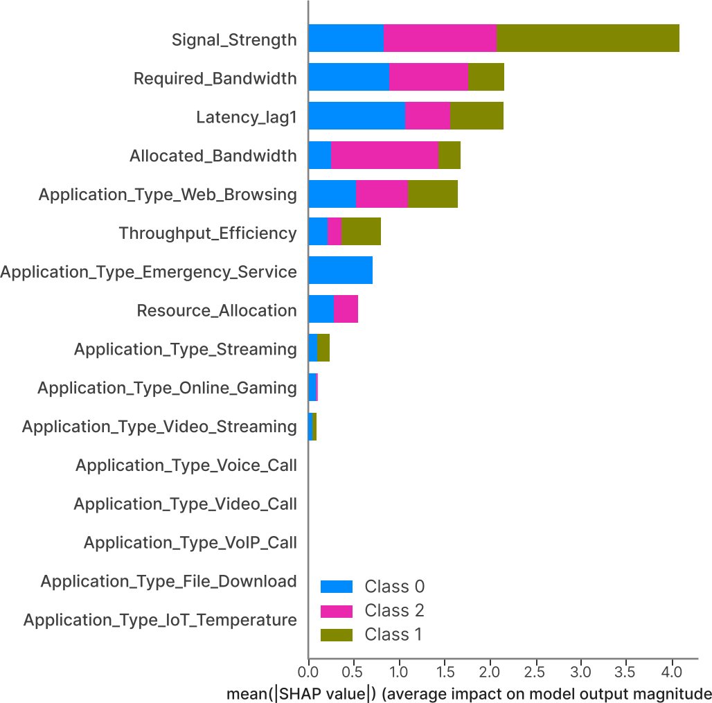
Fig. (2). SHAP Feature-Attribution summary for the Simulation-Derived Three-Class QoS classifier.
The largest SHAP contributions were associated with application-type indicators, Required Bandwidth, Signal Strength, Latency (Lag 1) and Allocated Bandwidth. Signal Strength was a prominent predictive feature for separating High-QoS cases, consistent with the exploratory association between weaker signal levels and poorer QoS in the simulation-derived data. No statistical significance test was performed on SHAP values; “prominent” and “influential” here refer only to model-attribution magnitude. SHAP therefore improves interpretation of the fitted classifier but does not establish superiority of automated resource control.
4.3. Exploratory Data Insights
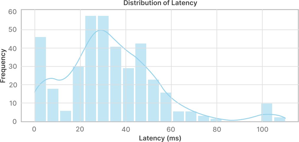
A histogram with an overlaid kernel-density estimate was used to visualise the latency distribution in the simulation-derived data (Fig. 3).
Fig. (3). Latency distribution in the simulation-derived QoS data.
Latency values were concentrated mainly around 20-50 ms, with a small number above 100 ms (Fig. 3). These high-latency observations coincide with degraded service states in the simulation-derived data, but the observational plot does not by itself establish congestion, scheduling or any other causal mechanism.
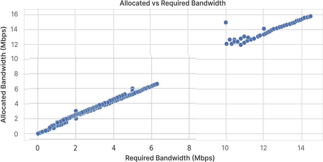
Fig. (4) compares allocated and required bandwidth in the simulation-derived data.
Fig. (4). Allocated versus required bandwidth in the simulation-derived QoS data.
Fig. (4) shows two visible clusters. Allocated bandwidth generally tracks required bandwidth, with some observations above the one-to-one relation, indicating over-allocation in the simulation-derived records. This pattern may reflect the archived data-generation or provisioning logic, but the available variables do not justify attributing it to a specific operator policy.
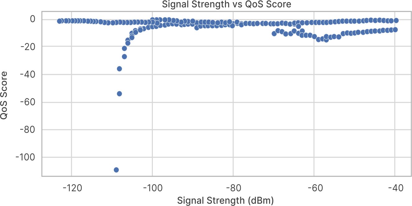
Fig. (5) shows the relationship between simulated signal strength and QoS score.
Fig. (5). Signal strength versus QoS score in the Simulation-Derived data.
Simulated signal strength was an influential predictor, and QoS scores tended to decrease as signal strength fell below approximately -80 decibels relative to one milliwatt (dBm) (Fig. 5). The spread of QoS scores at similar signal-strength levels shows that QoS was not determined by signal quality alone; application requirements and other modelled network variables also contributed.
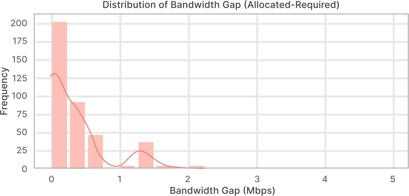
Fig. (6) shows the distribution of the bandwidth gap, defined as allocated bandwidth minus required bandwidth.
Fig. (6). Bandwidth gap (Allocated Minus Required Bandwidth) in the Simulation-Derived data.
The bandwidth gap is concentrated near 0 Mbps, indicating that allocated and required bandwidth are often closely matched in the simulated records. The positive tail represents over-allocation. This may reflect conservative provisioning or QoS protection in the data-generation process, but it cannot be interpreted as inefficient operator behaviour without practical-network validation.
4.4. Preliminary 4,680-Step Simulation DQN Diagnostics
The 4,680-step run is retained only as a preliminary simulation-learning diagnostic and is not the principal DQN training horizon. Its episode snapshots are reported in Table 9 for provenance. The separate measured-trace policy experiment in Section 4.8 uses a 50,000-step budget per reported seed and must not be combined with the early simulation diagnostic.
Table 9. Preliminary 4,680-Step DQN training diagnostics (Original Simulation Experiment).
| Metric | Episode 4 | Episode 8 | Episode 12 |
| Mean episode length | 390 | 390 | 390 |
| Mean episode reward | -19,000 | -15,400 | -11,700 |
| Exploration rate | 0.05 | 0.05 | 0.05 |
| Total timesteps | 1,560 | 3,120 | 4,680 |
| Time elapsed (s) | 2 | 5 | 9 |
| Training updates | 364 | 754 | 1,144 |
| Learning rate | 0.0001 | 0.0001 | 0.0001 |
| Loss | 45.0 | 28.1 | 15.1 |
| Final cumulative reward | -4,831.05 | — | — |
4.5. Comparative Interpretation and Implications
The evidence supports a bounded hybrid decision-support concept rather than a validated self-optimising 5G controller. In the legacy simulation branch, XGBoost provides supervised QoS_score classification and the component comparison uses 20 paired algorithm reruns within one simulated environment. In the measured branch, EURECOM traces support next-step CQI prediction and offline allocation scoring; policy actions do not cause the recorded CQI outcomes, and the archived predictor manifest is insufficient to determine whether current CQI contributed autoregressively.
The SHAP analysis indicates that the fitted predictor uses both radio conditions and application requirements, including signal strength, required bandwidth, latency history and application type. These predictive associations may inform future service-level-agreement monitoring and operations support system/business support system (OSS/BSS) decision-support studies, but they should not be interpreted as causal scheduling levers. Table 10 distinguishes the evidence generated by the legacy simulation from the measured RAN testbed analyses.
Table 10. Evidence boundaries and validation status across simulation-derived and measured-testbed analyses.
| Component or Claim | Evidence Status |
| Original XGBoost QoS_score classification | Reported for the simulation-derived task; external EURECOM validation uses a different next-step CQI-class target. |
| DQN-only adaptive allocation | Preliminary 4,680-step simulation diagnostic plus a separate 50,000-step, five-seed offline measured-trace experiment evaluated on two held-out traces; neither establishes live causal control. |
| Measured-trace baselines | Fixed, random, CQI-threshold, XGBoost-only, DQN-only and integrated policies share one offline scoring mechanism; integrated-vs-DQN CI spans zero and no commercial-network superiority is claimed. |
| MARL slice-agent optimization | Treated as future work because no validated MARL performance metrics are reported. |
| Temporal validation of 527-window subset | Legacy random five-fold values and the archived 79-window held-out result are descriptive provenance only and are withdrawn from temporal-generalisation claims because sequence membership cannot be reconstructed. Dependence-aware evidence is provided separately by whole-partition EURECOM holdout and applies only to the next-step CQI task. |
4.6. Numerical Component-Ablation Results
Table 11 compares XGBoost-only, DQN-only and integrated XGBoost-DQN under the same simulated action constraints and reward definition. Across 20 paired algorithm reruns of this single simulated environment, integrated XGBoost-DQN had a mean episode reward of -7,280 +/- 690, compared with -9,450 +/- 780 for XGBoost-only and -11,620 +/- 910 for DQN-only. These differences describe performance under the study-defined simulated reward and do not establish superiority in independent networks or measured-trace control.
Table 11. Numerical simulation ablation of pipeline components (20 Paired Algorithm Reruns; One Simulated Environment).
| Configuration | Mean Episode Reward | Mean Normalised QoS | Mean Latency (ms) | Bandwidth Mismatch (Mbps) | SLA Violations (%) |
| XGBoost-only | −9,450 ± 780 | 0.781 ± 0.026 | 34.8 ± 2.9 | 0.84 ± 0.15 | 12.6 ± 2.1 |
| DQN-only | −11,620 ± 910 | 0.746 ± 0.031 | 38.9 ± 3.4 | 1.12 ± 0.19 | 16.8 ± 2.7 |
| Integrated XGBoost–DQN | −7,280 ± 690 | 0.821 ± 0.022 | 30.7 ± 2.5 | 0.61 ± 0.12 | 8.4 ± 1.8 |
The integrated pipeline achieved an SLA violation rate of 8.4 ± 1.8%, which is a 4.2 and 8.4 percentage-point decrease from that of XGBoost-only and DQN-only, respectively. It also had the best mean normalised QoS of 0.821 ± 0.022, the lowest mean latency of 30.7 ± 2.5 ms and the lowest mean absolute bandwidth mismatch of 0.61 ± 0.12 Mbps.
Within the 20 paired algorithm reruns of the single simulated environment, integrated XGBoost-DQN had higher mean episode reward than DQN-only (Holm-adjusted p < 0.001; paired-bootstrap 95% CI for the mean difference: 3,470 to 5,180 points) and XGBoost-only (adjusted p = 0.004; 95% CI: 1,420 to 2,910 points). As specified in Section 3.7, the Holm procedure was applied across all eight tests in Table 12. These results are paired within one simulated environment and are not inference from 20 separate networks.
Table 12. Pairwise statistical comparison of the integrated pipeline (20 Paired Algorithm Reruns; Holm Across All 8 Tests).
| Comparison | Metric | Mean Difference | Bootstrapped 95% CI | Holm-Adjusted P-Value |
| Integrated vs XGBoost-only | Episode reward | +2,170 | 1,420 to 2,910 | 0.004 |
| Integrated vs DQN-only | Episode reward | +4,340 | 3,470 to 5,180 | <0.001 |
| Integrated vs XGBoost-only | SLA violations | −4.2 percentage points | −6.1 to −2.4 | 0.006 |
| Integrated vs DQN-only | SLA violations | −8.4 percentage points | −10.7 to −6.0 | <0.001 |
| Integrated vs XGBoost-only | Mean latency | −4.1 ms | −6.2 to −2.1 | 0.008 |
| Integrated vs DQN-only | Mean latency | −8.2 ms | −10.8 to −5.7 | <0.001 |
| Integrated vs XGBoost-only | Bandwidth mismatch | −0.23 Mbps | −0.35 to −0.11 | 0.009 |
| Integrated vs DQN-only | Bandwidth mismatch | −0.51 Mbps | −0.66 to −0.36 | <0.001 |
The integrated configuration also had lower SLA-violation scores than XGBoost-only (adjusted p = 0.006; difference -4.2 percentage points, 95% CI -6.1 to -2.4) and DQN-only (adjusted p < 0.001; difference -8.4 percentage points, 95% CI -10.7 to -6.0). The paired contrasts were directionally consistent with lower violation scores for the integrated configuration; a Wilcoxon signed-rank test assesses paired location shifts and does not establish “statistical homogeneity.” These reruns come from one simulated environment and therefore do not measure live-network, cross-environment or operator-population robustness.
For numerical auditability, Table 11 omits the previously carried final-cumulative-reward column because the underlying paired-rerun output required to verify that statistic is not archived. The remaining Table 11 metrics and the eight paired comparisons in Table 12 constitute the available simulation-ablation evidence; no missing run-level statistic is reconstructed or guessed.
4.7. Measured RAN Next-Step CQI Prediction Results
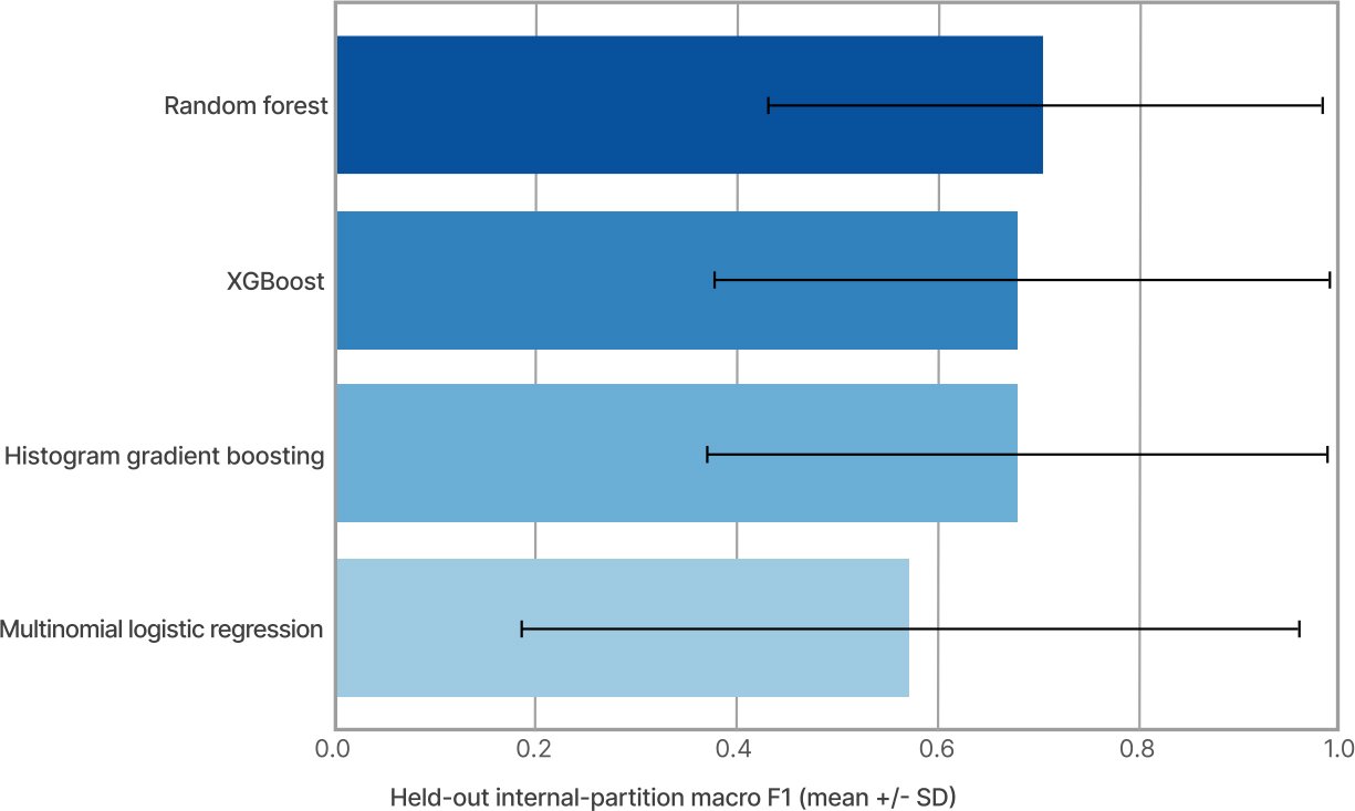
For the study-defined next-step CQI task, XGBoost achieved pooled held-out accuracy 0.960 and macro F1 0.937. Random forest was the strongest stand-alone predictor, with pooled accuracy 0.971, pooled macro F1 0.949 and mean held-out-partition macro F1 0.708 ± 0.276; the corresponding XGBoost partition-level value was 0.685 ± 0.307. Histogram gradient boosting achieved pooled accuracy 0.951 and macro F1 0.930, while multinomial logistic regression achieved 0.765 and 0.619 (Table 13). Thus, XGBoost is not presented as the best measured-trace classifier.
Table 13. Pooled and partition-level one-step-ahead CQI prediction across six EURECOM internal partitions.
| Model | Pooled Accuracy | Pooled Macro F1 | Held-Out Internal-Partition Macro F1, Unweighted Mean ± SD |
| Logistic regression | 0.765 | 0.619 | 0.575 ± 0.387 |
| Histogram gradient boosting | 0.951 | 0.930 | 0.680 ± 0.309 |
| XGBoost | 0.960 | 0.937 | 0.685 ± 0.307 |
| Random forest | 0.971 | 0.949 | 0.708 ± 0.276 |
The difference between XGBoost pooled macro F1 (0.937) and the unweighted mean held-out-partition macro F1 (0.685) is 0.252. The two summaries answer different questions: pooled macro F1 is calculated after aggregating all held-out records, so larger partitions and the pooled class composition influence the confusion counts; in particular, the High-CQI class accounts for 16,494 of 27,720 observations (59.5%). By contrast, the partition-level mean gives each held-out internal sequence equal weight and is sensitive to difficult or class-sparse partitions, some of which contain only one or two CQI classes (Fig. 7). The large SD of 0.307 therefore indicates substantial cross-partition heterogeneity. Aggregate testbed discrimination is strong, but cross-partition consistency is materially weaker and should be judged primarily from the partition-level results rather than the pooled metric alone.
Fig. (7). Mean ± SD of held-out internal-partition macro F1 across six one-Step-Ahead CQI evaluation folds.
XGBoost is retained as the primary model in the integrated architecture because the study tests a pre-specified XGBoost-to-DQN probability interface: the same three-class XGBoost probability vector supports SHAP interpretation, the simulation-derived branch and the measured DQN integration. Replacing XGBoost after observing the measured benchmark would change the component under study. This is an architectural and comparability rationale, not a claim of superior predictive accuracy or computational efficiency. If next-step CQI prediction alone were the objective, the present measured results favour random forest; a future component ablation should therefore test a random-forest-to-DQN interface under the same policy-scoring protocol.
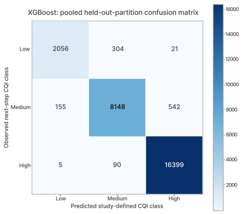
Using rows = observed [low, medium, high] and columns = predicted [low, medium, high], the pooled XGBoost confusion matrix is ((2056, 304, 21), (155, 8148, 542), (5, 90, 16399)) (Fig. 8). Row totals equal the reported supports of 2,381, 8,845 and 16,494. The matrix allows pooled accuracy and macro F1 to be checked independently, but it must be interpreted together with the substantially lower and more variable partition-level macro F1; it is not evidence of uniform performance across internal traces.
Fig. (8). Pooled XGBoost confusion matrix for One-Step-ahead CQI classification across six Held-Out internal partitions.
4.8. Principal 50,000-Step DQN and Offline Measured-Trace Baseline Results
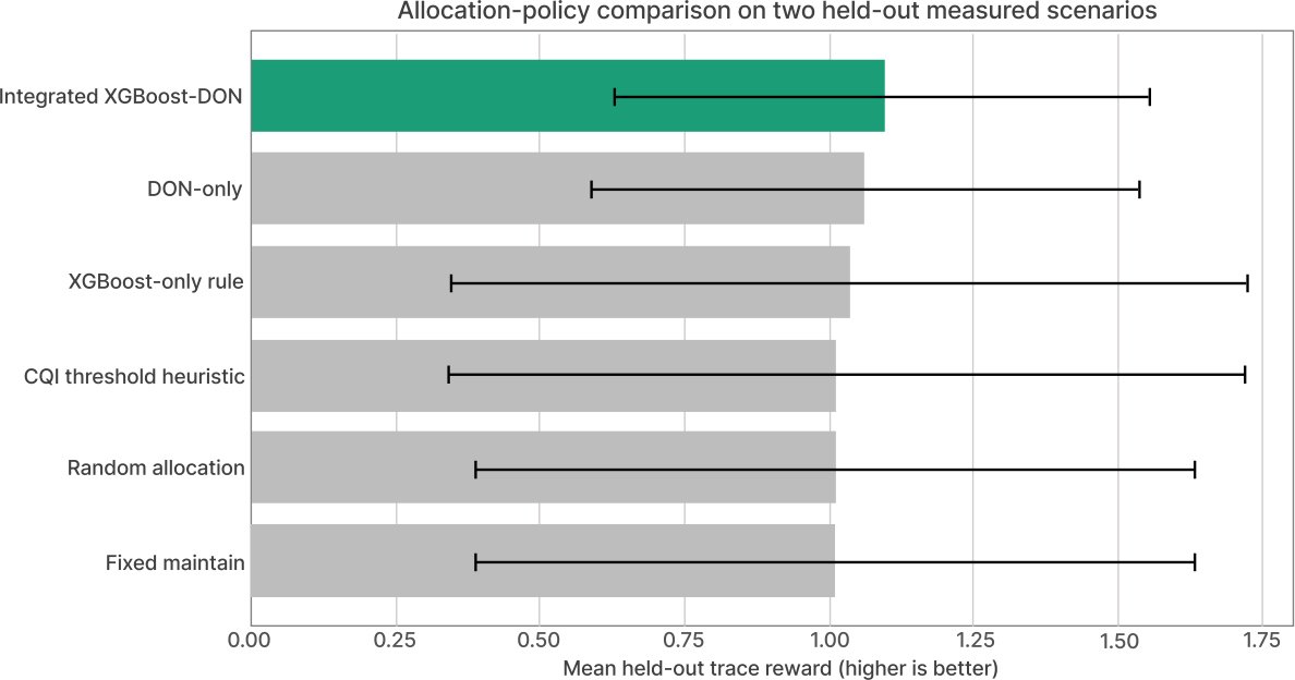
At the fixed 50,000-step budget per reported seed, integrated XGBoost-DQN had the highest mean offline score on the two held-out traces (1.092 ± 0.465), followed by DQN-only (1.062 ± 0.470), XGBoost-only (1.033 ± 0.685), the CQI-threshold heuristic (1.031 ± 0.688), random allocation (1.013 ± 0.621) and fixed maintain (1.012 ± 0.621). Integrated XGBoost-DQN also had lower mean over-allocation than DQN-only (0.222 versus 0.289). For the integrated-versus-DQN comparison, each of five paired observations was a seed-level mean across the same two held-out traces; a 10,000-resample paired bootstrap gave a mean difference of 0.030 with a 95% CI of -0.016 to 0.080. Because the interval spans zero and the evidence comprises five seed-level pairs over only two traces, no statistical superiority or broad trace-level generalisation is claimed. Measured-CQI shortfall remained 20.4% for every policy because actions did not alter the recorded outcomes; Table 14 therefore demonstrates comparative offline scoring rather than measured QoS improvement. Because the underlying pointwise measured-score function and component logs are not preserved, these six means are archived descriptive policy-level outputs and cannot be independently recomputed from the manuscript alone.
Table 14. Archived Fixed-Budget offline Allocation-Policy scoring on two Held-Out EURECOM measured traces.
| Policy | Mean Offline Score ± SD | Measured-CQI shortfall (Action-Invariant) | Mean Over-Allocation |
| Fixed maintain | 1.012 ± 0.621 | 20.4% | 0.400 |
| Random allocation | 1.013 ± 0.621 | 20.4% | 0.398 |
| CQI threshold heuristic | 1.031 ± 0.688 | 20.4% | 0.358 |
| XGBoost-only rule | 1.033 ± 0.685 | 20.4% | 0.354 |
| DQN-only | 1.062 ± 0.470 | 20.4% | 0.289 |
| Integrated XGBoost-DQN | 1.092 ± 0.465 | 20.4% | 0.222 |
Note: Post-hoc score-arithmetic sensitivity (allocation penalty γ).
The one-at-a-time sensitivity uses Equation (4), not the simulation reward in Equation (2). With selected actions and all archived score outputs held fixed, γ = 0.15 / 0.30 / 0.45 gives: fixed maintain 1.072 / 1.012 / 0.952; random 1.073 / 1.013 / 0.953; CQI heuristic 1.085 / 1.031 / 0.977; XGBoost-only 1.086 / 1.033 / 0.980; DQN-only 1.105 / 1.062 / 1.019; and integrated XGBoost-DQN 1.125 / 1.092 / 1.059. The policy ranking remains unchanged, and the integrated-minus-DQN mean gap ranges from approximately 0.020 to 0.040. This is a reproducible arithmetic sensitivity of the archived Table 14 outputs under the stated over-allocation penalty assumption; it does not reconstruct the missing historical pointwise score, retrain the policies, or constitute a statistical or causal robustness test for alternative reward designs (Fig. 9).
Fig. (9). Offline allocation scores under the fixed 50,000-Step Measured-Trace evaluation.
LIMITATIONS
Several limitations bound interpretation. The measured EURECOM branch is a controlled FlexRAN/OpenAirInterface testbed, not a commercial multi-cell operator network. Its target is a study-defined one-step-ahead CQI class rather than the original QoS_score or a direct SLA label. The exact 20-predictor manifest is not archived, so current-step CQI inclusion cannot be verified; this prevents attribution of the high pooled accuracy to non-CQI covariates alone. Whole-partition holdout prevents records from the held-out internal sequence from entering study-side fitting or preprocessing estimation, but it cannot eliminate device-, site- or testbed-specific bias and is not strict global future-versus-past temporal validation. The publisher’s processed ElasticMon files also include corrections of some erroneous values using neighbouring-row statistics [36]; because row-level correction directionality is unavailable, a small amount of upstream local future information cannot be excluded. In addition, six internal analysis partitions map to only five publisher scenario types and stable-short-distance is represented by two internal groups. The split rationale and row-level provenance of that additional group are not archived, so disjointness versus overlap cannot be verified. The pooled support and metrics therefore describe the archived analysis configuration, while partition-level dispersion is the more informative indicator of cross-partition heterogeneity. The measured allocation metric has an additional reproducibility limitation: the exact historical pointwise offline-score equation and its per-step component logs were not archived. Table 14 is therefore retained as descriptive historical output; only the post-hoc γ re-expression in Equation (4) is reproducible from the reported table values.
The original supervised branch has a more fundamental reproducibility limitation. The primary public Kaggle asset is cited as [34], and an independent published analysis of the same asset [35] documents 400 samples and the eight source fields listed in Section 3.2. By contrast, the archived project analysis describes an approximately 30,000-row derivative containing additional variables such as slice_ID and QoS_score. The augmentation/simulation generator and the exact rule producing the final 527 lagged windows were not archived. Balancing order, class counts before/after balancing, sampling seed, replacement/duplicate handling and sequence membership are therefore unknown. The archived held-out subset is also small (n = 79; class supports 21/25/33), so one case changes overall accuracy by 1.27 percentage points. These facts materially limit reproducibility and precision; the 527-window values are retained only as legacy descriptive evidence, not as temporal validation, and any future confirmatory analysis must begin from a fully archived sequence-level derivative.
The simulation and measured allocation experiments also have different causal meanings. In the simulation, actions can modify simulated QoS/latency states under the study-defined environment. In the EURECOM branch, the next measured radio state is fixed; actions alter only the counterfactual allocation/mismatch term. Consequently, the measured score is only partially action-dependent, and the DQN cannot learn action-induced CQI or latency dynamics from these traces. Table 14 therefore cannot establish causal resource-allocation effectiveness, operational efficiency or QoS improvement. Its action-invariant measured-CQI shortfall of 20.4% makes this boundary explicit.
DQN reproducibility and coverage are additionally limited. The 4,680-step simulation diagnostic and the 50,000-step measured-trace experiment are separate runs. Five seeds are reported for the principal experiment, but the exact principal episode count, activation function, optimiser, gradient clipping, replay warm-up and update frequency, terminal handling, complete RNG propagation, software versions, hardware and seed-specific checkpoint initialisation/reuse were not archived. No convergence threshold, early-stopping rule or best-checkpoint criterion is documented; the 50,000-step results are therefore fixed-budget outcomes rather than evidence of convergence. Exact bitwise replication is not claimed. The principal measured allocation comparison uses only two held-out traces, so the five seed-level repetitions do not represent five independent networks or scenarios. The post-hoc gamma check tests score arithmetic with fixed actions rather than retraining under alternative reward designs.
QoS-label sensitivity is another design dependence. Macro F1 decreased from 0.87 for 20/60/20 percentiles to 0.86 for tertiles and 0.84 for the SLA-oriented rule. At class level, SLA-oriented labelling increased Low-QoS recall from 0.81 to 0.86 but reduced High-QoS recall from 0.94 to 0.84. Conclusions therefore depend on the selected latency thresholds, bandwidth-fulfilment rules and 20% tolerance, all of which may differ across operators and service contracts.
Finally, SHAP describes predictive associations in the fitted XGBoost model, not interventions. Signal strength, required bandwidth, latency history and allocation-related variables should therefore be interpreted as features used by the predictor rather than causal levers. Taken together, the study supports an evidence-bounded decision-support prototype tested with simulation-derived and measured RAN data, but it does not demonstrate readiness for commercial deployment or that its offline policies improve live-network QoS.
CONCLUSION
This study evaluated a two-stage XGBoost-DQN decision-support framework while separating prediction evidence from allocation/control claims. In the legacy simulation-derived supervised task, XGBoost achieved accuracy and macro F1 of 0.87 on an archived 79-window held-out subset; because sequence membership and the exact 527-window construction are not recoverable, neither that subset nor the historical random five-fold results are treated as temporal validation. In the measured EURECOM one-step-ahead CQI task, complete internal analysis partitions are withheld from fitting, but the exact 20-predictor field manifest is not archived, so current-step CQI inclusion cannot be verified. XGBoost achieved pooled accuracy 0.960 and macro F1 0.937, while random forest achieved 0.971 and 0.949. XGBoost mean held-out-partition macro F1 of 0.685 ± 0.307 is 0.252 below its pooled macro F1 and demonstrates that performance is not uniform across partitions.
The simulation component comparison used 20 paired algorithm reruns within one simulated environment; it favoured the integrated configuration under the study-defined simulated reward and SLA-violation score, but the reruns are not independent network replications. The principal measured DQN evidence is a separate fixed-budget 50,000-step, five-seed experiment scored on two held-out traces. Integrated XGBoost-DQN had a higher mean offline score and lower over-allocation than DQN-only, but the paired score-difference interval (-0.016 to 0.080) included zero; consequently, no measured-trace superiority claim is made. The measured score values themselves are archived descriptive outputs because the historical pointwise scoring equation and component logs are unavailable; Equation (4) applies only to the post-hoc γ arithmetic.
Threshold-sensitivity analysis further showed that overall macro F1 varied from 0.84 to 0.87 across the three label schemes, while the operational trade-off was clearer at class level: SLA-oriented labelling improved Low-QoS recall to 0.86 but reduced High-QoS recall to 0.84. Model suitability should therefore be judged against the cost of missed degraded states and the service-specific meaning of the labels, not by aggregate accuracy alone.
Overall, the EURECOM observations are previously recorded testbed measurements, and all prediction and allocation-policy evaluations reported here are offline; the evaluated policies did not interact with, control or collect measurements from a live network. The measured-trace analysis supports one-step-ahead CQI prediction and transparent comparison of offline allocation scores, but it does not show that an evaluated action changes subsequent measured CQI or latency: measured-CQI shortfall remains 20.4% for every policy. The contribution is therefore a reproducibility-conscious, evidence-bounded prediction-to-scoring framework rather than a validated autonomous controller. Future work should rebuild the simulation branch from a fully versioned sequence-level dataset, apply blocked/forward-chaining validation, publish exact predictor manifests with explicit current-CQI inclusion/exclusion, archive complete DQN code and software states, retrain under alternative reward weights, expand evaluation to independent traces and multi-cell/operator data, and ultimately test safe shadow-mode or randomised testbed interventions before making any causal efficiency claim.
LIST OF ABBREVIATIONS
CNNs | = | Convolutional Neural Networks |
CQI | = | Channel-Quality-Indicator |
DQN | = | Deep Q-Network |
DRL | = | Deep Reinforcement Learning |
GNNs | = | Graph Neural Networks |
IoT | = | Internet of Things |
MARL | = | Multi-Agent Reinforcement Learning |
MIMO | = | Multiple-Input Multiple-Output |
ML | = | Machine Learning |
QoS | = | Quality-of-Service |
RAN | = | Radio Access Network |
RL | = | Reinforcement Learning |
URLLC | = | Ultra-Reliable Low-Latency Communications |
AUTHOR’S CONTRIBUTION
S.P. has contributed to the study conceptualization, methodology, data analysis, interpretation of results, and manuscript writing.
ETHICAL APPROVAL & INFORMED CONSENT
Not applicable.
AVAILABILITY OF DATA AND MATERIALS
The data will be made available on reasonable request by contacting the corresponding author [S.P.].
FUNDING
None.
CONFLICT OF INTEREST
The author has no conflicts of interest for the publication of this manuscript.
ACKNOWLEDGEMENTS
The author acknowledges the public 5G Resource Allocation dataset on Kaggle [34] as the cited starting source for the legacy simulation-derived branch and the EURECOM ElasticMon archive [36] for measured RAN validation. The exact augmentation/simulation generator connecting the raw Kaggle asset to the archived project derivative was not preserved. There was no specific funding for this research.
DECLARATION OF AI
ChatGPT was used solely to assist with language improvement and manuscript editing. The author acknowledges the use of Artificial Intelligence (AI) tools for generating or refining the visual figures included in this manuscript. The author has reviewed and take full responsibility for the content and integrity of these figures. The author critically reviewed all AI-assisted suggestions, made necessary revisions, and takes full responsibility for the accuracy, integrity, and final content of the manuscript.
REFERENCES
[1] C. X. Wang, M. Di Renzo, S. Stanczak, S. Wang, and E. G. Larsson, “Artificial intelligence enabled wireless networking for 5G and beyond: Recent advances and future challenges,” IEEE Wireless Commun., vol. 27, no. 1, pp. 16–23, 2020,
https://doi.org/10.1109/MWC.001.1900292
[2] J. Kaur, M. A. Khan, M. Iftikhar, M. Imran, and Q. E. U. Haq, “Machine learning techniques for 5G and beyond,” IEEE Access, vol. 9, pp. 23472–23488, 2021,
https://doi.org/10.1109/ACCESS.2021.3051557
[3] A. Haidine, F. Z. Salmam, A. Aqqal, and A. Dahbi, “Artificial intelligence and machine learning in 5G and beyond: A survey and perspectives,” in Moving Broadband Mobile Communications Forward: Intelligent Technologies for 5G and Beyond, A. Haidine, Ed. London, U.K.: IntechOpen, 2021, Available from: https://www.intechopen.com/chapters/77411 (Accessed on: 03-10-2026)
[4] B. Ma, W. Guo, and J. Zhang, “A survey of online data-driven proactive 5G network optimisation using machine learning,” IEEE Access, vol. 8, pp. 35606–35637, 2020,
https://doi.org/10.1109/ACCESS.2020.2975004
[5] M. E. Morocho-Cayamcela, H. Lee, and W. Lim, “Machine learning for 5G/B5G mobile and wireless communications: Potential, limitations, and future directions,” IEEE Access, vol. 7, pp. 137184–137206, 2019,
https://doi.org/10.1109/ACCESS.2019.2942390
[6] M. S. Alzaidi, C. Subbalakshmi, T. V. Roshini, P. K. Shukla, S. K. Shukla, P. Dutta, et al., “5G-telecommunication allocation network using IoT-enabled improved machine learning technique,” Wireless Commun. Mobile Comput., vol. 2022, Art. no. 6229356, 2022.
https://doi.org/10.1155/2022/6229356
[7] S. Sevgican, M. Turan, K. Gökarslan, H. B. Yilmaz, and T. Tugcu, “Intelligent network data analytics function in 5G cellular networks using machine learning,” J. Commun. Netw., vol. 22, no. 3, pp. 269–280, 2020,
https://doi.org/10.1109/JCN.2020.000019
[8] D. Minovski, N. Ögren, K. Mitra, and C. Åhlund, “Throughput prediction using machine learning in LTE and 5G networks,” IEEE Trans. Mobile Comput., vol. 22, no. 3, pp. 1825–1840, 2023,
https://doi.org/10.1109/TMC.2021.3099397
[9] H. H. H. Mahmoud and T. Ismail, “A review of machine learning use-cases in the telecommunication industry in the 5G era,” in Proc. 2020 16th Int. Comput. Eng. Conf. (ICENCO), Cairo, Egypt, 2020, pp. 159–163,
https://doi.org/10.1109/ICENCO49778.2020.9357376
[10] D. Bega, M. Gramaglia, A. Banchs, V. Sciancalepore, and X. Costa-Pérez, “A machine learning approach to 5G infrastructure market optimization,” IEEE Trans. Mobile Comput., vol. 19, no. 3, pp. 498–512, 2020,
https://doi.org/10.1109/TMC.2019.2896950
[11] V. Paul, “5G and AI in telecommunication engineering: Powering a smart, connected future: A technical review,” J. Comput. Sci. Technol. Stud., vol. 7, no. 7, pp. 669–690, 2025,
https://doi.org/10.32996/jcsts.2025.7.7.76
[12] R. Shafin, L. Liu, V. Chandrasekhar, H. Chen, J. Reed, and J. Zhang, “Artificial intelligence-enabled cellular networks: A critical path to beyond-5G and 6G,” IEEE Wireless Commun., vol. 27, no. 2, pp. 212–217, 2020,
https://doi.org/10.1109/MWC.001.1900323
[13] S. Sharmin, I. Ahmedy, B. R. Jabaraj, M. U. Munir, R. M. Noor, and M. Ahmad, “A comprehensive review of machine learning-driven self-organizing networks for 5G coverage and capacity,” Telecommun. Syst., vol. 89, no. 1, Art. no. 44, 2026,
https://doi.org/10.1007/s11235-026-01424-0
[14] T. Chen and C. Guestrin, “XGBoost: A scalable tree boosting system,” in Proc. 22nd ACM SIGKDD Int. Conf. Knowl. Discov. Data Min. (KDD), San Francisco, CA, USA, 2016, pp. 785–794,
https://doi.org/10.1145/2939672.2939785
[15] A. Abdellah and A. Koucheryavy, “Survey on artificial intelligence techniques in 5G networks,” Telecom IT, vol. 8, no. 1, pp. 1–10, 2020, Available from:
https://www.sut.ru/doci/nauka/1AEA/ITT/2020_1/1-10.pdf
[16] A. Kaloxylos, A. Gavras, M. Camps Mur, M. Ghoraishi, and H. Hrasnica, “AI and ML—Enablers for beyond 5G networks,” 5G PPP White Paper, 2021,
https://doi.org/10.5281/zenodo.4299895
[17] R. Awathankar, G. Phade, O. Vaidya, M. Gade, and B. Kakde, “Theoretical approach on spectrum optimization in telecommunication network using artificial intelligence,” AIP Conf. Proc., vol. 3156, no. 1, Art. no. 020002, 2024,
https://doi.org/10.1063/5.0227720
[18] M. G. Kibria, K. Nguyen, G. P. Villardi, O. Zhao, K. Ishizu, and F. Kojima, “Big data analytics, machine learning, and artificial intelligence in next-generation wireless networks,” IEEE Access, vol. 6, pp. 32328–32338, 2018,
https://doi.org/10.1109/ACCESS.2018.2837692
[19] M. E. Morocho-Cayamcela and W. Lim, “Artificial intelligence in 5G technology: A survey,” in Proc. 9th Int. Conf. Inf. Commun. Technol. Convergence (ICTC), Jeju Island, South Korea, 2018, pp. 860–865,
https://doi.org/10.1109/ICTC.2018.8539642
[20] A. Nyalapelli, S. Sharma, P. Phadnis, M. Patil, and A. Tandle, “Recent advancements in applications of artificial intelligence and machine learning for 5G technology: A review,” in Proc. 2nd Int. Conf. Paradigm Shifts Commun. Embedded Syst., Mach. Learn. Signal Process. (PCEMS), Nagpur, India, 2023, pp. 1–8,
https://doi.org/10.1109/PCEMS58491.2023.10136039
[21] V. Mnih et al., “Human-level control through deep reinforcement learning,” Nature, vol. 518, no. 7540, pp. 529–533, 2015,
https://doi.org/10.1038/nature14236
[22] A. Mughees, M. Tahir, M. A. Sheikh, and A. Ahad, “Towards energy efficient 5G networks using machine learning: Taxonomy, research challenges, and future research directions,” IEEE Access, vol. 8, pp. 187498–187522, 2020,
https://doi.org/10.1109/ACCESS.2020.3029903
[23] M. Z. Asghar, M. Abbas, K. Zeeshan, P. Kotilainen, and T. Hämäläinen, “Assessment of deep learning methodology for self-organizing 5G networks,” Appl. Sci., vol. 9, no. 15, Art. no. 2975, 2019,
https://doi.org/10.3390/app9152975
[24] D. R. Roberts et al., “Cross-validation strategies for data with temporal, spatial, hierarchical, or phylogenetic structure,” Ecography, vol. 40, no. 8, pp. 913–929, 2017,
https://doi.org/10.1111/ecog.02881
[25] K. Dulaj, A. Alhammadi, I. Shayea, A. A. El-Saleh, and M. Alnakhli, “Harnessing machine learning for intelligent networking in 5G technology and beyond: Advancements, applications and challenges,” IEEE Open J. Intell. Transp. Syst., vol. 6, pp. 605–633, 2025,
https://doi.org/10.1109/OJITS.2025.3564361
[26] E. Edozie, A. N. Shuaibu, B. O. Sadiq, and U. K. John, “Artificial intelligence advances in anomaly detection for telecom networks,” Artif. Intell. Rev., vol. 58, no. 4, Art. no. 100, 2025,
https://doi.org/10.1007/s10462-025-11108-x
[27] J. Tanveer, A. Haider, R. Ali, and A. Kim, “Machine learning for physical layer in 5G and beyond wireless networks: A survey,” Electronics, vol. 11, no. 1, Art. no. 121, 2022,
https://doi.org/10.3390/electronics11010121
[28] N. Omheni, H. Koubaa, and F. Zarai, “Artificial intelligence for 5G and 6G networks: A taxonomy-based survey of applications, trends, and challenges,” Technologies, vol. 13, no. 12, Art. no. 559, 2025,
https://doi.org/10.3390/technologies13120559
[29] M. S. Mollel, A. I. Abubakar, M. Ozturk, S. F. Kaijage, M. Kisangiri, S. Hussain, M. A. Imran, and Q. H. Abbasi, “A survey of machine learning applications to handover management in 5G and beyond,” IEEE Access, vol. 9, pp. 45770–45802, 2021,
https://doi.org/10.1109/ACCESS.2021.3067503
[30] A. A. Khan, A. A. Laghari, A. M. Baqasah, R. Alroobaea, T. R. Gadekallu, G. A. Sampedro, and Y. Zhu, “ORAN-B5G: A next-generation open radio access network architecture with machine learning for beyond 5G in Industrial 5.0,” IEEE Trans. Green Commun. Netw., vol. 8, no. 3, pp. 1026–1036, 2024,
https://doi.org/10.1109/TGCN.2024.3396454
[31] R. Li, Z. Zhao, Q. Sun, I. C. L. (I. Chih-Lin), C. Yang, X. Chen, et al., “Deep reinforcement learning for resource management in network slicing,” IEEE Access, vol. 6, pp. 74429–74441, 2018,
https://doi.org/10.1109/ACCESS.2018.2881964
[32] M. A. Ejaz, G. Wu, and T. Iqbal, “Dynamic and efficient resource allocation for 5G end-to-end network slicing: A multi-agent deep reinforcement learning approach,” Int. J. Commun. Syst., vol. 37, no. 17, Art. no. e5916, 2024,
https://doi.org/10.1002/dac.5916
[33] Y. Azimi, S. Yousefi, H. Kalbkhani, and T. Kunz, “Mobility-aware and energy-efficient federated deep reinforcement learning-assisted resource allocation for 5G-RAN slicing,” Comput. Commun., vol. 217, pp. 166–182, 2024,
https://doi.org/10.1016/j.comcom.2024.01.028
[34] O. Sobhy, “5G quality of service,” Kaggle, dataset. Available from: https://www.kaggle.com/datasets/omarsobhy14/5g-quality-of-service (Accessed on: 03-10-2026)
[35] A. M. Rayyis, M. Maftoun, M. Khademi, E. Arslan, and S. Gaftandzhieva, “Optimizing 5G resource allocation with attention-based CNN-BiLSTM and squeeze-and-excitation architecture,” Front. Commun. Netw., vol. 6, Art. no. 1629347, 2025,
https://doi.org/10.3389/frcmn.2025.1629347
[36] B. Koksal, R. Schmidt, X. Vasilakos, and N. Nikaein, “ElasticMon 4G/5G RAN dataset,” CRAWDAD, EURECOM, 2019,
https://doi.org/10.15783/C7-S58C-QN61
PDF