Information and Uncertainty Analysis of the OBXII-IRD Using Seven Measures of Entropy with Application to Carbon Fibers Data

Article DOI 10.67887/PD2601208008

📚 Cited by: 0

⬇ Downloads: 37

Authors

Alaa A. Khalaf^1,*
, Mundher A. Khaleel^2,
, Ahmed M. Salih^2,
, Ali T. Mohammed^3,
, Moudher Kh. Abdal-Hammed^4,
, Qasim N. Husain^5,

¹Ministry of Education, Diyala Education Directorate, Diyala, Iraq

²Department of Mathematics, College of Computer Science and Mathematics, Tikrit University, Tikrit, Iraq

³Department of Mathematics College of Education for Pure Sciences (Ibn AL-Haitham), University of Baghdad, Iraq

⁴Department of public Administration, Collage of Administration and Economics, Tikrit University, Tikrit, Iraq

⁵Department of Mathematics, College of Education for Pure Science, University of Tikrit, Iraq

Article History:

Received: 04 January, 2026

Accepted: 16 July, 2026

Revised: 14 July, 2026

Published: 01 October, 2026

ABSTRACT:

Introduction: This research studies the Odd Burr Inverse Rayleigh (OBXII-IRD) distribution, concentrating on parameter estimation methods and entropy measures.

Methodology: Three estimation methods: Maximum likelihood estimation, maximum product of spacings, and Kolmogorov were used and their outcomes were investigated using Monte Carlo simulation.

Results: The results demonstrated their ability to estimate parameters reasonably well. Seven entropy measures including Renyi, Shannon, Tsallis, Arimoto, Havrda-Charvat, Sharma-Mittal, and Sant’ Anna-Taneja were subject to distribution’s uncertainty. To show its practical perfomance, the OBXII-IRD was utilized to real-world data representing carbon fibers.

Conclusion: The results indicate that the OBXII-IRD is superior and fits the data better than other distributions. The statistical software R was used for all programming and computational tasks in this study.

Keywords: Inverse rayleigh distribution, non-bayesian estimation, MLE, information criterion, goodness-of-fit statistics, carbon fibers.

1. INTRODUCTION

Trayer [1] introduced the inverse Rayleigh distribution model for checking the reliability and survival data, as followed by Voda [2], whom investigated the distribution’s basic properties and acknowledged the potential for approximating the lifetime distribution of experimental units. Later, Graf [3] compared the parameter estimators for inverse Rayleigh and derived five measures of location the arithmetic, harmonic, and geometric means, as well as the mode and median.

Howlader et al., [4] determined Bayesian prediction limits for lifetime models based on the inverse Rayleigh distribution. Banerjee and Bohoni [5] introduced the exponentiated transformed inverse Rayleigh distribution and investigated various estimation methods. Khan and King [6] addressed the Transmuted modified inverse Rayleigh distribution and explored its statistical properties. Meanwhile, Goual and Yousef [7] proposed a modified inverse Rayleigh based on the Burr XII distribution, originally introduced by Cordeiro et al. [8] contributing to the study of its mathematical properties and associated regression model. Ali [9] study the inverse Rayleigh distribution mixture, determined its properties, and employed Bayesian estimation to estimate its parameters.

Fisher [10] and Rao [11] established the framework for weighted distributions, while Aydin [12] introduced the weighted inverse Rayleigh distribution, their comprehensive study of the mathematical properties of these distributions contributed to a better understanding of weighted distributions in statistical analysis. For further information on exponential and weighted distributions, as well as Bayesian estimation methods, please refer to the sources [13–17].

Cover and Thomas [18] provided a comprehensive foundation for information theory, building upon the work of Shannon [19], who established the concept of entropy to measure uncertainty. To explore different types of entropy, consult see the refer [20–25].

In this article, we extend the Odd Burr XII- inverse Rayleigh distribution, for which Khalaf et al., [26] established statistical characteristics and estimated parameters via the maximum likelihood estimation, by introducing the following novel contributions:

First, present three different classical methods for estimating the parameters of the OBXII-IR distribution, employing various sample sizes to ensure numerical consistency and methodological robustness.

Secondly, as our core theoretical contribution, we provide a thorough evaluation of uncertainty from an information-theoretic standpoint and compelling inaugural seven diverse generalized entropy measures, thereby providing a comprehensive and unprecedented characterization of model randomness from multiple mathematical viewpoints.

In the end, we investigate the practical implication of the model using real-world engineering data from materials science (carbon fibers) to present our developed estimation and entropy frameworks providing superior and highly competitive modeling in contrast to other leading distributions.

The rest of the paper is sectioned into 7 sections. Section 2 contains the mathematical part of the probability density function and the cumulative distribution function for the OBXII-IR distribution. Section 3 demonstrates the informational area by evaluating seven different measures of entropy to quantify the uncertainty in the model. Section 4 reviews the three estimation methods used to extract the parameters of the distribution, followed by Section 5, investigates the intensive simulation experiments to evaluate the efficiency of these estimators. In Section 6, real world implication is discussed, and lastly in Section 7 concludes the study.

2. THE ODD BURR INVERSE RAYLEIGH (OBXII-IRD) DISTRIBUTION

Below are the cumulative distribution (cdf) and density function (pdf) of the OBXII-IR distribution Eq: (1 & 2):

where .

Fig. (1) depicts the probability density function (pdf) of the OBXII-IRD under different combinations of shape and scale parameters, reflecting the high structural flexibility of the model in modeling real data:

Fig. (1). Pdf plot for OBXII-IRD.

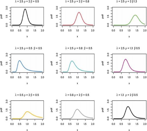
Effect of the β parameter (first line): When the parameters (λ = 2.5, ρ = 2) are held constant and the value of the scale parameter β is increased from 0.5 to 1.3, a clear shift of the function’s curve to the right is observed, along with an increase in the curve’s flattening and the extension of its tail.
In terms of the shape parameter and its behavior as the parameter increases, while keeping constant. At low values, we observe that the curve’s skewness is positive; as the value of beta increases, the function becomes steeper.
In terms of the shape parameter and its behavior as the parameter increases from 0.5 to 1.3, while keeping constant observe the peak becoming sharper and the horizontal spread of the curve contracting, this indicates that acts as a shape parameter, controlling the expansion and contraction of the function.

Fig. (2) illustrates the behavior of the cumulative distribution function (cdf) for the proposed OBXII-IRD. All curves reflect the standard mathematical properties of any continuous and true cumulative distribution function:

Fig. (2). Cdf plot for OBXII-IRD.

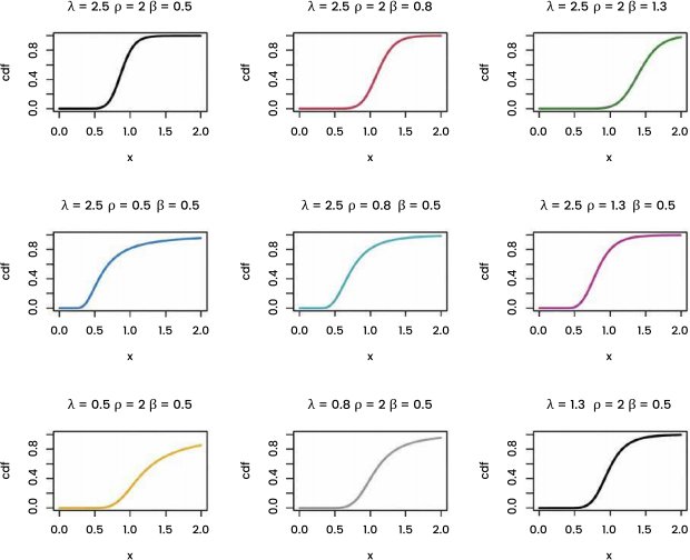
Checking the mathematical boundary conditions: It is clearly shown from all the graphs that the function starts precisely from zero at the minimum space , and increases monotonically, continuously and smoothly to reach the maximum integer one , thus proving the mathematical validity of the deduced equations.
The elasticity of S-shaped curves: The cumulative function takes on elastic forms, oscillating between sharp arrowhead curves and soft S-shaped curves, depending on the parameter values. We observe that as the values of the parameters β and λ increase, the function becomes more concave and the later it reaches one, which perfectly matches the heavy-tail behavior observed in the corresponding PDF graphs in Fig. (1).

3. VARIOUS ENTROPY MEASURES

As mentioned in the introduction, the entropy of the OBXII-IRD can be measured in various ways. This allows for the analysis and understanding of the uncertainty in the OBXII-IRD, and such analyses are important in machine learning and information theory. Due to the complexity of the OBXII-IRD function, the equations cannot be written in closed form; therefore, they are expressed as integrals and can be calculated numerically or using an Arithmetic programming language.

3.1. Rényi Entropy

The Renyi entropy is considered a generalization of Shannon entropy and serves as an important measure of uncertainty for probability distribution, the dispersion of data in OBXII-IRD can be described using the order parameter. It can be expressed by the following equation Eq (3):

Substituting equation (2) into the integrand yields

3.2. Shannon Entropy

Shannon entropy is one of the most widely used measures of dispersion in information theory, and for the OBXII-IRD, it can use the following formula Eq (4):

Using (2), can be derived

3.3. Tsallis Entropy

The entropy Tsallis of the OBXII-IRD is calculated using the following formula Eq (5):

Substituting equation (2) into the integrand obtain:

3.4. Arimoto Entropy

Arimoto entropy prosses a highly flexible formula for handling complex probability distribution, therefore, it is considered a fundamental measure in information theory. It can be calculated for the OBXII-IRD using the following equation:

From (2) we obtain Eq (6):

3.5. Havrda and Charvat Entropy

The Havrda-Charvat measure was introduced as a generalized of Shannon entropy to account for changes in probability distribution. It is significant for describing in complex systems via the order parameter . For the OBXII-IRD. It is calculated using the following equation Eq (7):

provided by (2):

3.6. Sharma and Mittals Entropy

Sharma and Mittal entropy is one of the most comprehensive and flexible information measures, developed as a general framework combining the properties of Rennie and Tsalis entropy. Sharma and Mittal entropy is calculated using the following equation Eq (8):

From equation (2) we get:

3.7. Sant’ Anna and Taneja Entropy

The Sant’ Anna-Taneja entropy measure as it combines two entropy concepts to confirm a stabilize analysis subject to uncertainty. It is highly potent for measuring data sensitive to dispersion and described the OBXII-IRD by the following equation Eq (9):

By equation (2), we obtain:

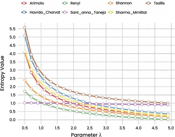
Tables 1, 2, and 3 shows an in-depth evaluation of the seven entropy measures for the OBXII-IRD, presenting the degree of uncertainty as the distribution’s shape and scale parameters differs.

Table 1. Analysis of different entropy values for the OBXII-IRD assuming that ρ =1.1, β =2, and α=0.8.

λ	SE	TE	RE	AE	HCE	SME	STE
0.5	2.3860396	5.5776488	1.7187630	4.0902935	5.0895332	4.1128168	1.0219391
0.7	1.8671114	3.9367975	1.3703675	2.8508409	3.6178475	3.0444185	1.0174308
0.9	1.5419278	3.1139745	1.1358997	2.2091862	2.8353101	2.4292448	1.0123078
1.1	1.3138240	2.6211115	0.9636036	1.8082477	2.3381825	2.0210105	1.0068136
1.3	1.1423852	2.2925825	0.8296745	1.5299954	1.9891350	1.7262145	1.0011308
1.5	1.0072308	2.0573765	0.7214324	1.3234421	1.7277609	1.5010252	0.9953748
1.7	0.8973578	1.8802082	0.6313708	1.1627522	1.5230172	1.3219408	0.9895968
1.9	0.8052719	1.7415690	0.5547875	1.0333551	1.3572151	1.1751999	0.9838479
2.1	0.7267437	1.6298520	0.4884836	0.9263445	1.2194554	1.0520836	0.9781567
2.3	0.6586215	1.5376947	0.4302848	0.8359762	1.1026659	0.9468542	0.9725333
2.5	0.5987558	1.4602081	0.3785708	0.7583545	1.0019886	0.8555280	0.9669901
2.7	0.5455279	1.3940054	0.3321890	0.6907479	0.9140263	0.7752578	0.9615580
2.9	0.4977599	1.3367153	0.2902172	0.6311488	0.8362773	0.7039466	0.9562022
3.1	0.4545450	1.2856464	0.2519654	0.5780798	0.7668881	0.6400042	0.9509409
3.3	0.4151652	1.2422077	0.2126866	0.5304220	0.7044360	0.5822346	0.9457827
3.5	0.3790688	1.2026692	0.1845321	0.4873055	0.6478110	0.5296678	0.9407178
3.7	0.3457878	1.1671505	0.1545611	0.4480388	0.5961452	0.4815494	0.9357408
3.9	0.3149657	1.1305476	0.1266689	0.4120632	0.5487383	0.4372581	0.9308567
4.1	0.2862955	1.1058445	0.1006014	0.3789305	0.5050104	0.3963070	0.9260633
4.3	0.2595136	1.0791452	0.0761680	0.3482951	0.4645155	0.3582786	0.9213524
4.5	0.2344365	1.0546235	0.0531870	0.3198231	0.4268364	0.3228197	0.9167352
4.7	0.2108477	1.0319989	0.0314973	0.2932810	0.3916669	0.2896583	0.9121970
4.9	0.1886097	1.0110460	0.0109821	0.2684505	0.3589187	0.2585233	0.9077211

Table 2. Analysis of different entropy values for the OBXII-IRD assuming that λ=0.6, β=2.5, and α=0.8.

Ρ	SE	TE	RE	AE	HCE	SME	STE
0.5	3.6169382	9.8069901	2.2830950	9.1668579	10.718397	7.1379715	1.0249472
0.7	2.9503923	7.7673642	2.0499307	5.8309067	7.0826555	5.4077942	1.0241710
0.9	2.5183360	6.2375193	1.8305828	4.3919402	5.4406382	4.403415	1.0229331
1.1	2.2033291	5.1373630	1.6365399	3.5586635	4.4642482	3.7239238	1.0212614
1.3	1.9572714	4.3338714	1.4664616	2.9998814	3.7874623	3.2221629	1.0191607
1.5	1.7562455	3.7310175	1.3166804	2.5910908	3.3029147	2.8301676	1.0166272
1.7	1.5867686	3.2662962	1.1836565	2.2744467	2.9156225	2.5117163	1.0136615
1.9	1.4405394	2.8992346	1.0644462	2.0191386	2.6005008	2.2454941	1.0102648
2.1	1.3121122	2.6031082	0.9567068	1.8071003	2.3367529	2.0180154	1.0064353
2.3	1.1977243	2.3598114	0.8585813	1.6269621	2.1111657	1.8202677	1.0021786
2.5	1.0946781	2.1567477	0.7686006	1.4711630	1.9148933	1.6459578	0.9974959
2.7	1.0009745	1.9849368	0.6855869	1.3344552	1.7417480	1.4905399	0.9923917
2.9	0.9150917	1.8378339	0.6085877	1.2130625	1.5872561	1.3506296	0.9869705
3.1	0.8358498	1.7105663	0.5368244	1.1041904	1.4480864	1.2236255	0.9809393
3.3	0.7623119	1.5994471	0.4696571	1.0057188	1.3216977	1.1076024	0.9746031
3.5	0.6937246	1.5016334	0.4065532	0.9160027	1.2061145	1.0008911	0.9678695
3.7	0.6294724	1.4149042	0.3470613	0.8337472	1.0997727	0.9022462	0.9607459
3.9	0.5690472	1.3375016	0.2908032	0.7579153	1.0014128	0.8106250	0.9532396
4.1	0.5120243	1.2680152	0.2374520	0.6876634	0.9100103	0.7251721	0.9453595
4.3	0.4580451	1.2053044	0.1867311	0.6222978	0.8247196	0.6451743	0.9371134
4.5	0.4068045	1.1484338	0.1383984	0.5612429	0.7448349	0.5700297	0.9285121
4.7	0.3580408	1.0966317	0.0922435	0.5040132	0.6697617	0.4992278	0.9195655
4.9	0.3115262	1.0492552	0.0480807	0.4502020	0.5989984	0.4323339	0.9102819

Table 3. Analysis of different entropy values for the OBXII-IRD assuming that λ=0.9, ρ=1.1, and α=0.8.

β	SE	TE	RE	AE	HCE	SME	STE
0.5	0.8487740	1.5569854	0.4427510	1.2212801	1.5977375	1.2442260	0.9689681
0.7	1.0170102	1.8422506	0.6109873	1.4455652	1.8825392	1.5168312	0.9852560
0.9	1.1426673	2.0889156	0.7366449	1.6193504	2.1016019	1.7266883	0.9944222
1.1	1.2430024	2.3093829	0.8369808	1.7620870	2.2805157	1.8980020	1.0002993
1.3	1.3265305	2.5105635	0.9205076	1.8836756	2.4322208	2.0432634	1.0043874
1.5	1.3980804	2.6967774	0.9920577	1.9898669	2.5642035	2.1696403	1.0073965
1.7	1.4606626	2.8709396	1.0546395	2.0843177	2.6812004	2.2816686	1.0097036
1.9	1.5162744	3.0351232	1.1102512	2.1695008	2.7864053	2.3824055	1.0115288
2.1	1.5663166	3.1908704	1.1602935	2.2471679	2.8820774	2.4740138	1.0130087
2.3	1.6118025	3.3393613	1.2057798	2.3186124	2.9698730	2.5580807	1.0142324
2.5	1.6534934	3.4815250	1.2474702	2.3848142	3.0510492	2.6358088	1.0152611
2.7	1.6919733	3.6181062	1.2859503	2.4465337	3.1265772	2.7081277	1.0161392
2.9	1.7277039	3.7497174	1.3216800	2.5043742	3.1972277	2.7757776	1.0168965
3.1	1.7610487	3.8768629	1.3550261	2.5588238	3.2636214	2.8393514	1.0175568
3.3	1.7923098	3.9999678	1.3862860	2.6102822	3.3262669	2.8993352	1.0181369
3.5	1.8217299	4.1193959	1.4157061	2.6590806	3.3855838	2.9561321	1.0186516
3.7	1.8495148	4.2354573	1.4434910	2.7054977	3.4419247	3.0100803	1.0191093
3.9	1.8758362	4.3484230	1.4698136	2.7497678	3.4955886	3.0614658	1.0195212
4.1	1.9008412	4.4585776	1.4948184	2.7920949	3.5468293	3.1105300	1.0198933
4.3	1.9246553	4.5659770	1.5186328	2.8326520	3.5958690	3.1574863	1.0202314
4.5	1.9473864	4.6709551	1.5413637	2.8715912	3.6428975	3.2025174	1.0205836
4.7	1.9691296	4.7736264	1.5631068	2.9090441	3.6880802	3.2457819	1.0208207
4.9	1.9899658	4.8741341	1.5839429	2.9451286	3.7315651	3.2874197	1.0210789

First: Table 1 shows the conduct of the seven entropy and its result of slowly increasing the value of while keeping the parameters fixed and .

From the Table 1 and Fig. (3), we inspect that all seven entropy measures decrease with increasing For example, Reny entropy values decline abruptly from 1.1787 at to 0.0109 at , and likewise, STE entropy decreases from 1.0219391 to 0.9077211.
From a mathematical point of view, we notice that the PDF constrict and reduces as the value of the parameter This geometric outcome shows a decline in data dispersion, signifying a decrease in the system’s level of uncertainty.

Fig. (3). It illustrates the behavior of entropy measures and their changes at different values of the parameter λ.

Second: Table 2 depicts the behavior of the seven entropy and effect of gradually increasing the value of while keeping the parameters fixed and .

From the Table 2 and Fig. (4), we observe that all seven entropy measures decrease with increasing value. For example, Shannon entropy values decline sharply from 3.6169382 at to 0.3115262 at .

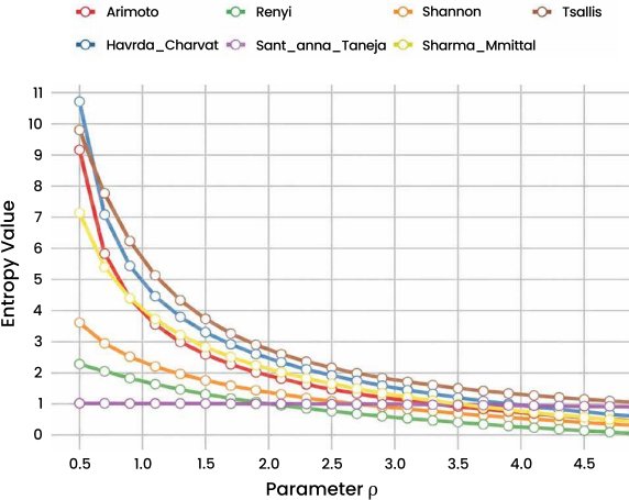
Fig. (4). It illustrates the behavior of entropy measures and their changes at different values of the parameter ρ.

From a mathematical view point, it’s been observed that the PDF constrict and cinch as the parameter surge, resulting in data clustering around the model. This geometric inclination proposes a decrease in data dispersion, which indicates a lower degree of uncertainty in the system.

Third: Table 3 displays the behavior of the seven entropies and the impact of slowly increasing the value of while maintaining fixed values for and α=0.8.

Table 3 and Fig. (5) show that when the value increases, each of the seven entropy measures decrease. Arimoto entropy values, for instance, decrease dramatically from 1.2212801 at =0.5 to 2.9451286 at =4.9.

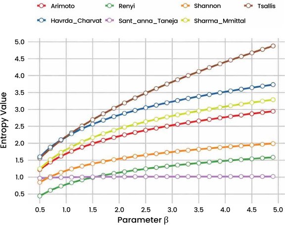
Fig. (5). It illustrates the behavior of entropy measures and their changes at different values of the parameter β.

Regarding the statistical interpretation, we observe that the situation for the parameter beta differs from that of the parameters here, increasing the values of led to an increase in all entropy measures due to the heightened randomness of the system and the dispersion of the data.

Key Conclusions: All seven entropy measures showed complete consistency and logical agreement in their response to changes in the parameters of the OBXII-IRD, thus proving the mathematical stability of the model. Rényi entropy and Shannon entropy are the most sensitive and ideal in detecting and characterizing these dynamic shifts with extreme accuracy compared to the Sant’Anna-Taneja (ST) measure, which showed a slow response and very slight changes around the value (1).

4. NON-BAYESIAN ESTIMATION METHODS

This section reviews the classical inference methods for estimating the parameters of the OBXII-IRD, which include: Maximum Likelihood Estimation (MLE), Approximate Confidence Interval (ACI), Maximum Product space Estimation (MPS), and Kolmogorov Estimation (KE).

This section will identify the Inference Classica estimators for the OBXII-IRD parameter set .

4.1. MLE

Let be a random sample of size n drawn from the OBXII-IRD; accordingly, the Likelihood Function denoted by L according to the sources [28–31], can be expressed as follows Eq: (10).

The derivation of the log-likelihood function for is as follows Eq: (11).

The potential log-likelihood function is partially derived with respect to the coefficients to obtain the maximum potential estimators Eq: (12 & 13).

Where solve three equations at the same time to get an approximation for λ, ρ, and β. The integral of becomes zero when also becomes zero. Using statistical software like R, one may achieve the necessary results.

4.1.1. ACI

Here we examine the most common confidence intervals; the asymptotic properties of MLEs were used to calculate the range of confidence intervals at a significance level of 100(1 – α) % for the unknown parameters λ, ρ, and β. If the regularity conditions are met, the MLEs follow a normal asymptotic distribution with a mean of (λ, ρ, β) and a variance-covariance matrix represented by , i.e., that:

Assuming the existence of a variance and covariance matrix, denoted by:

The asymptotic variances for λ, ρ, and β.are determined by the elements on the main diagonal of the matrix. Accordingly, confidence intervals at a significance level of 100(1 – α) % for λ, ρ, and β can be calculated using normal approximation according to the following equations:

4.2. MPSE

It minimizes the MPS function to estimate λ, σ, and β for further details on MPS, see to [32].

From equation (1) we get Eq: (15).

4.3. KE

The Kolmogorov estimation is used in the process of estimating the parameters for the OBXII-IRD. The object of this estimating method is to find the minimum value of the following equation [33].

From equation (1) we get Eq: (16).

5. SIMULATION

To assess the statistical effectiveness and numerical efficiency of the different estimation methods proposed in Section (5) for the OBXII-IRD, a detailed Monte Carlo simulation study was introduced. This study was formulated to ensure the accuracy and reproducibility of the results by integrating the following methodological aspects:

Number of Replications: N = 1000 independent random samples were originated for each simulated scenario to maintain the stability of the estimates and minimize random error.
Testing five different sample sizes, namely:30, 60, 120, 200, and 300.
True parameter values:

Group 1: (λ= 0.7, ρ=3.2, β=1.1).

Group 2: (λ= 0.7, ρ=3, β=0.8).

Group 3:( λ= 0.8, ρ=3.5, β=1.2).

To examine the properties of the estimators, three cases were selected with different values of skewness, kurtosis, and measures of dispersion. This variation ensures an assessment of the robustness of the estimation methods for the OBXII-IRD.

5.1. Statistical Evaluation Metrics

1. The numerical average (Mean):

Mean=

2. Bias: Measures the range to which the estimated value deviates from the true value:

Bias =

3. Root Mean Square Error (RMSE):

RMSE =

4. Convergent Confidence Intervals (ACI): Confidence intervals were calculated at a significance level of 95% using the observed information matrix.

5. Average interval length (AIL): Measures how narrow and useful the confidence interval is (the shorter the interval, the more accurate the estimate):

AIL=

6. Probability of Convergence (CP): Measures the proportion of times (out of 1000 iterations) that the confidence interval successfully contained the true value of the parameter θ.

where : is actual value of the parameter, : estimated value of the parameter, and i: is iteration number.

Based on this methodology, estimation methods were tested to determine the optimal and most appropriate option for modeling real data, and the numerical results and trends will be reviewed in detail in the following tables.

Our modeling findings are sensibly reported in Tables 4–6. Additionally, we have skillfully visualized the numerical data in these tables. Lower positions indicate more strength and dominance in this situation. These classifications measure the performance of each estimation method. The Table provide a comprehensive overview of the effectiveness and strengths of the estimation methods associated with the various approaches.

Table.4. Simulation results for the OBXII-IRD parameter estimators at λ= 0.7, ρ=3.2, β=1.1.

N	–	E. P.	MLE	MPSE	KE	–	MLE	MPSE	KE
30	Mean		1.622832	1.670051	0.874213	ACI	0.201573 5.997310	0.110347 6.593772	0.094540 1.653886
			3.618142	3.979477	3.332589		0.342760 8.576670	0.014837 10.70739	1.536750 5.128428
			1.790221	2.107840	1.142415		0.290987 4.814944	0.104590 5.623921	0.843442 1.441388
	RMSE		2.781051	3.072686	0.460859	AIL	5.997310	6.593772	1.559345
			2.678373	3.577665	0.976439		8.576670	10.707393	3.591677
			1.891007	2.351347	0.166341		4.184944	5.623921	0.597945
	Bias		0.922832	0.970051	0.174213	CP	90.90	91.70	95.90
			0.418142	0.779477	0.132589		96.10	96.30	95.40
			0.690221	1.007840	0.042415		92	89.50	95.10
60	Mean		1.034505	1.046923	0.803711	ACI	0.257890 3.734370	0.270166 3.948830	0.250642 1.356780
			3.466517	3.587803	3.292458		0.595910 6.337125	0.065259 7.110348	1.931589 4.653327
			1.322467	1.475725	1.127753		0.390142 3.067305	0.230197 3.821698	0.877966 1.377539
	RMSE		1.661849	1.627603	0.338568	AIL	3.734370	3.948830	1.106138
			1.683450	1.896067	0.758210		5.741215	7.045089	2.721737
			1.058683	1.408452	0.132393		3.067305	3.821698	0.499572
	Bias		0.334505	0.346923	0.103711	CP	97.40	97.40	94.40
			0.266517	0.387803	0.092458		95.50	97.40	93.80
			0.222467	0.375725	0.027753		96.20	93.90	95.10
120	Mean		0.829646	0.868709	0.761395	ACI	0.280124 2.459609	0.301275 2.663477	0.323185 1.199605
			3.268995	3.335976	3.250479		1.963295 4.574695	1.939246 4.732705	2.092412 4.408546
			1.153148	1.184195	1.119303		0.416327 1.889969	0.294774 2.073615	0.953626 1.284980
	RMSE		0.865512	0.968270	0.247901	AIL	2.459609	2.663477	0.876419
			0.732288	0.817622	0.599500		2.611399	2.793458	2.316133
			0.387601	0.543503	0.101619		1.473642	1.778840	0.331353
	Bias		0.129646	0.168709	0.061395	CP	99.40	98.70	94.60
			0.068995	0.135976	0.050479		93.20	92.60	94.50
			0.053148	0.084195	0.019303		99.40	99.10	91.10
200	Mean		0.745958	0.761770	0.742843	ACI	0.302968 1.188948	0.323754 1.199786	0.342542 1.143143
			3.230426	3.270664	3.230080		2.393511 4.067340	2.378038 4.163291	2.324641 4.135519
			1.117921	1.125003	1.113685		0.946407 1.289435	0.930309 1.319697	0.953471 1.273899
	RMSE		0.233947	0.259318	0.210393	AIL	0.885979	0.876031	0.800601
			0.501349	0.533272	0.491025		1.673829	1.785253	1.810878
			0.098419	0.106175	0.085612		0.343027	0.389387	0.320427
	Bias		0.045958	0.061770	0.042843	CP	95.40	94.40	94.80
			0.030426	0.070664	0.030080		91.50	91.70	93.30
			0.017921	0.025003	0.013685		94	94.60	94
300	Mean		0.721551	0.731162	0.734181	ACI	0.416339 1.026762	0.422068 1.040255	0.422579 1.045784
			3.237158	3.266084	3.227192		2.546719 3.927596	2.456371 4.075798	2.409439 4.044945
			1.107873	1.112459	1.110635		0.973505 1.242241	0.969974 1.254944	0.961063 1.260207
	RMSE		0.163844	0.178128	0.188929	AIL	0.610422	0.618187	0.623205
			0.406883	0.429947	0.435941		1.380877	1.619427	1.635505
			0.075497	0.077047	0.078393		0.268736	0.284969	0.299144
	Bias		0.021551	0.031162	0.034181	CP	94.10	92.70	93.40
			0.027158	0.066084	0.027192		91	94.20	94.30
			0.007873	0.012459	0.010635		93	93.90	95.10

Table 5. Simulation results for the OBXII-IRD parameter estimators at λ= 0.7, ρ=3, β=0.8.

N	–	Est. Par.	MLE	MPSE	KE	–	MLE	MPSE	KE
30	Mean		1.770023	1.985029	0.879650	ACI	0.083715 6.393954	0.011204 7.455226	0.116109 1.643192
			3.406014	3.832228	3.109433		0.290347 8.174990	0.702398 11.80781	1.351819 4.867046
			1.290037	1.582152	0.834830		0.184204 3.359213	0.021457 4.181349	0.604868 1.064792
	RMSE		2.972387	3.484761	0.454819	AIL	6.393954	7.455226	1.527083
			2.576590	4.222474	0.953106		8.174990	11.80781	3.515226
			1.300242	1.754422	0.123525		3.359213	4.181349	0.459923
	Bias		1.070023	1.285029	0.179650	CP	90.20	88.90	95.20
			0.406014	0.832228	0.109433		96.20	97	95.10
			0.490037	0.782152	0.034830		92.10	89.80	95.30
60	Mean		1.052190	1.210251	0.808010	ACI	0.170390 3.669367	0.063788 4.955028	0.239749 1.376271
			3.244548	3.350994	3.085509		0.488223 6.000874	1.012487 6.748188	1.730357 4.440661
			0.985503	1.118970	0.823305		0.279934 2.328251	0.060237 2.974303	0.624842 1.021767
	RMSE		1.616805	2.114571	0.348314	AIL	3.669367	4.955028	1.136522
			1.614671	1.824029	0.754253		5.512650	6.748188	2.710304
			0.817839	1.119906	0.105460		2.328251	2.974303	0.396924
	Bias		0.352190	0.510251	0.108010	CP	96.70	95.60	95.10
			0.244548	0.350994	0.085509		96.70	97.40	93.70
			0.185503	0.318970	0.023305		95.60	93	95
120	Mean		0.822177	0.878648	0.767653	ACI	0.240321 2.156483	0.098732 2.620398	0.339574 1.195732
			3.063460	3.120998	3.022349		1.813244 4.313676	1.765536 4.476459	1.987373 4.057325
			0.839340	0.876177	0.817348		0.362339 1.316344	0.132213 1.620140	0.688134 0.946562
	RMSE		0.711099	0.942381	0.244185	AIL	2.156483	2.620398	0.886157
			0.700931	0.791716	0.534344		2.500423	2.710922	2.069952
			0.245164	0.455544	0.079722		0.954004	1.487927	0.298427
	Bias		0.122177	0.178648	0.067536	CP	99	98.80	93.60
			0.063460	0.120998	0.022349		93.10	92.50	94.20
			0.039341	0.076177	0.017348		99.10	98.80	91.60
200	Mean		0.748494	0.772209	0.748512	ACI	0.288772 1.208216	0.119433 1.424986	0.313089 1.183936
			3.027410	3.063039	3.026606		2.222836 3.831984	2.198354 3.927724	2.135948 3.917264
			0.814926	0.822505	0.812455		0.676776 0.953076	0.617802 1.027207	0.677128 0.947781
	RMSE		0.242941	0.382221	0.229250	AIL	0.919444	1.305552	0.870847
			0.481867	0.515890	0.482836		1.609147	1.729369	1.781316
			0.079365	0.110803	0.072461		0.276301	0.409405	0.270653
	Bias		0.048494	0.072209	0.048512	CP	95.80	97.20	95.40
			0.027410	0.063039	0.026606		91.40	91.70	93.30
			0.014926	0.022505	0.012455		94.10	97.30	95
300	Mean		0.718325	0.728446	0.735705	ACI	0.410950 1.025700	0.389956 1.066936	0.426551 1.044810
			3.052700	3.076489	3.016812		2.275297 3.825242	2.311706 3.841272	2.276289 3.757335
			0.804828	0.808625	0.808429		0.706218 0.903438	0.711219 0.906031	0.704036 0.91282
	RMSE		0.165297	0.178520	0.177168	AIL	0.614750	0.676980	0.61830
			0.405335	0.428302	0.400803		1.549944	1.529565	1.481045
			0.055601	0.059030	0.057354		0.197220	0.194811	0.208786
	Bias		0.018325	0.028446	0.035750	CP	94.70	95.70	92.60
			0.050270	0.076489	0.016812		93.90	92.20	92.80
			0.004828	0.008625	0.008429		93	92.40	93.30

Table 6. Simulation results for the OBXII-IRD parameter estimators at λ= 0.8, ρ=3.5, β=1.2.

N	–	E. P.	MLE	MPSE	KE	–	MLE	MPSE	KE
30	Mean		1.774507	1.488012	0.992217	ACI	0.096783 6.804978	0.037489 5.886295	0.140345 1.844090
			3.870576	4.314009	3.668577		0.991023 8.932019	0.078649 12.29458	1.755870 5.581285
			1.943762	2.298931	1.236282		0.192674 5.138058	0.078136 6.052449	0.946624 1.525941
	RMSE		3.170328	2.693662	0.504147	AIL	6.804978	5.886295	1.703744
			2.725754	4.221473	1.044050		8.932019	12.29458	3.825415
			2.002488	2.520089	0.159996		5.138058	6.052449	0.579316
	Bias		0.974507	0.688012	0.192217	CP	92.80	95.60	93.40
			0.370576	0.814009	0.168577		96.30	96.80	94.60
			0.743762	1.098931	0.036282		91.80	89.30	93.10
60	Mean		1.075368	1.094546	0.918114	ACI	0.101289 3.488727	0.060127 3.716324	0.257503 1.578725
			3.722728	3.848282	3.608937		1.269901 6.175555	0.294581 7.401983	2.123780 5.094093
			1.453770	1.637379	1.225184		0.360297 3.414366	0.172037 4.307581	0.975343 1.475025
	RMSE		1.480908	1.466563	0.402672	AIL	3.488727	3.716324	1.321221
			1.437662	1.904517	0.828476		4.905653	7.107401	2.970313
			1.190397	1.605732	0.131906		3.414366	4.307581	0.499681
	Bias		0.275368	0.294546	0.118111	CP	97.90	98	94.20
			0.222728	0.348282	0.108937		92.20	97.50	93.80
			0.253770	0.437379	0.025184		96.20	93.50	94.40
120	Mean		0.909620	0.935391	0.879270	ACI	0.240256 2.030847	0.096246 1.774536	0.369911 1.376030
			3.562273	3.623513	3.556115		2.202556 4.921989	2.175559 5.071467	2.319159 4.793072
			1.257299	1.289767	1.219103		0.435934 2.078663	0.352258 2.227275	1.051502 1.386704
	RMSE		0.598774	0.465895	0.285214	AIL	2.030847	1.678290	1.006118
			0.761740	0.844881	0.640528		2.719432	2.895907	2.473913
			0.431812	0.573048	0.102719		1.642728	1.875017	0.335201
	Bias		0.109620	0.135391	0.072970	CP	98.20	95.10	93.90
			0.062273	0.123513	0.056115		93.50	92.90	94.10
			0.057299	0.089767	0.019103		99.50	99.20	91.30
200	Mean		0.859797	0.884102	0.853816	ACI	0.323385 1.396209	0.348237 1.419968	0.392118 1.315515
			3.252544	3.560858	3.520731		2.653212 4.397277	2.633077 4.488639	2.593466 4.447996
			1.218963	1.227373	1.214774		1.043974 1.393952	1.028040 1.426706	1.052755 1.375799
	RMSE		0.284127	0.319388	0.243597	AIL	1.072823	1.071730	0.923396
			0.522034	0.552747	0.502345		1.744065	1.855561	1.854298
			0.100539	0.109137	0.086389		0.349978	0.398666	0.323044
	Bias		0.059797	0.084102	0.053816	CP	95.70	94.80	94.40
			0.0325244	0.060858	0.040731		91.40	91.90	92.50
			0.018963	0.027373	0.014277		94.10	95	93.50
300	Mean		0.827901	0.843225	0.832136	ACI	0.470419 01.185382	0.476654 1.209796	0.487849 1.176423
			3.534059	3.558983	3.536905		2.818367 4.249750	2.721176 4.396790	2.718194 4.355417
			1.208278	1.213908	1.207418		1.073331 1.343225	1.069948 1.357867	1.063687 1.351149
	RMSE		0.192271	0.212438	0.207802	AIL	0.714963	0.733142	0.688574
			0.421380	0.443517	0.437101		1.431382	1.675614	1.637222
			0.072850	0.078068	0.075003		0.269893	0.287919	0.287461
	Bias		0.027901	0.043225	0.032136	CP	94.40	93.30	92.20
			0.034059	0.058983	0.036805		91.30	94.20	94.20
			0.008278	0.013908	0.007418		93.10	93.60	94.90

Tables 4–6 provide a summary of the simulation results illustrating capability performance. The main conclusions can be summarized as follows:

7. All estimation converge toward the true parameter values as the value of n increases, confirming their consistency with respect to the parameters.

8. A decrease in bias value was observed for all methods as the sample size increased, indicating improved accuracy in estimating the parameters of the OBXII-IRD.

9. The results Table 7 and Fig. (6) demonstrated all methods achieved satisfactory performance; however, the best performing method was the KE method, which exhibited high accuracy and minimized the gap between theoretical and empirical distribution making it an effective alternative to MLE method.

Table 7. Results of the descriptive analysis of the data used.

Dataset	N	Mean	SD	Median	mad	Min	Max	Rang	CS	CK	SE
Data	100	1.66	0.6	1.54	0.4	0.92	5.31	4.39	3.13	14.08	0.06

Note: mad: Median Absolute Deviation; CS: Coefficient of Skewness; CK: Coefficient of Kurtosis; SE: Standard Error of the mean

Fig. (6). Display data and its representation.

6. APPLICATION

To demonstrate the applicability and high suitability of the OBXII-IRD, we compared it with three competing distributions (such as, IR, HLIR [34], and OFIR [35]). based on real carbon fiber data. Table 8 presents the maximum likelihood estimates (MLEs) for the model parameters, along with the quality of fit test statistics Cramér-von Mises )W(, Anderson-Darling (A) and Kolmogorov-Smirnov (K) with the probability value (P-value). Table 9 summarizes the integrated statistical trade-off criteria, which include the negative probability function value (-LL), Akaike Information Criteria, Consistent AIC, Bayesian Information Criteria, Hanan and Quinn.

Table 8. MLEs and differentiation criteria for various models.

Model	MLEs	W	A	KS	P-value
OBXII-IR	:8.981019 :0.138496 :2.544796	0.055622	0.427378	0.059803	0.866877
IR	:2.202159	0.086196	0.705385	0.325146
HLIR	:4.827274 :3.921237	0.139856	1.101967	0.080599	0.534419
OFIR	:1.296087 :1.551353	0.196541	1.302636	0.117163	0.128402

Table 9. Statistical preference criteria and quality of fit for the data set.

Model	-LL	AIC	CAIC	BIC	HQIC
OBXII-IR	51.83538	109.6708	109.9208	117.4863	112.8338
IR	89.86446	181.7289	181.7697	184.3341	182.7833
HLIR	57.17079	118.3416	118.4653	123.5519	120.4503
OFIR	57.37916	118.7583	118.8820	123.9680	120.8670

Based on the results in Tables 8 and 9, the superiority of the OBXII-IRD over the comparative distribution can be explained by the following reasons:

Table 8 shows that the OBXII-IRD recorded the smallest distance between the empirical and theoretical distributions in the KS specifically 0.059803, which is the lowest value among the competing distributions. This superiority is directly reflected in the P-value 0.866877, which exceeded the standard significance level (0.05), indicating a failure to reject the null hypothesis. Consequently, the proposed distribution offers a better fit for the data and outperforms the comparative distributions.
The OBXII-IRD also yields the lowest statistical values W= 0.055622 and A= 0.427378. this superiority minimizes the squared differences between the empirical and cdf thereby enhancing the model’s reliability at the extremes of the data.
Table 9 demonstrates the efficiency of the OBXII-IRd based on information criteria, it achieved the lowest values for (-LL=51.8353, AIC=109.67, BIC=117.48, and HQIC=112.83). consequently, the OBXII-IRD is considered the most suitable fit for the data compared to the other distributions evaluated, as the distribution yielding the lowest values for these criteria is deemed superior.

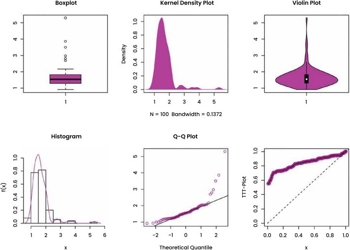
The study included breaking stress data for 100 carbon fibers, obtained from reference [36]

(0.92, 0.928, 0.997, 0.9971, 1.061, 1.117,1.162, 1.183, 1.187, 1.192, 1.196, 1.213, 1.215, 1.2199, 1.22, 1.224, 1.225, 1.228, 1.237, 1.24, 1.244, 1.259,1.261, 1.263, 1.276, 1.31, 1.321, 1.329, 1.331, 1.337,1.351, 1.359, 1.388, 1.408, 1.449, 1.4497, 1.45, 1.459, 1.471, 1.475, 1.477, 1.48, 1.489, 1.501, 1.507, 1.515,1.53, 1.5304, 1.533, 1.544, 1.5443, 1.552, 1.556, 1.562, 1.566, 1.585, 1.586, 1.599, 1.602, 1.614, 1.616, 1.617, 1.628, 1.684, 1.711, 1.718, 1.733, 1.738, 1.743, 1.759, 1.777, 1.794, 1.799, 1.806, 1.814, 1.816, 1.828, 1.83, 1.884, 1.892, 1.944, 1.972, 1.984, 1.987, 2.02, 2.0304, 2.029, 2.035, 2.037, 2.043, 2.046, 2.059, 2.111, 2.165, 2.686, 2.778, 2.972, 3.504, 3.863, 5.306).

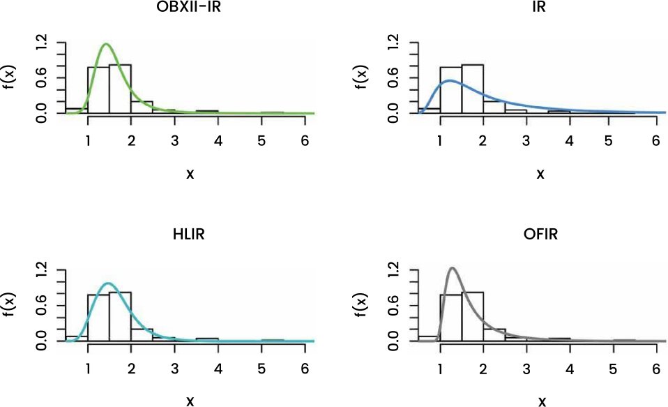
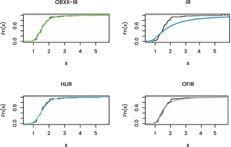
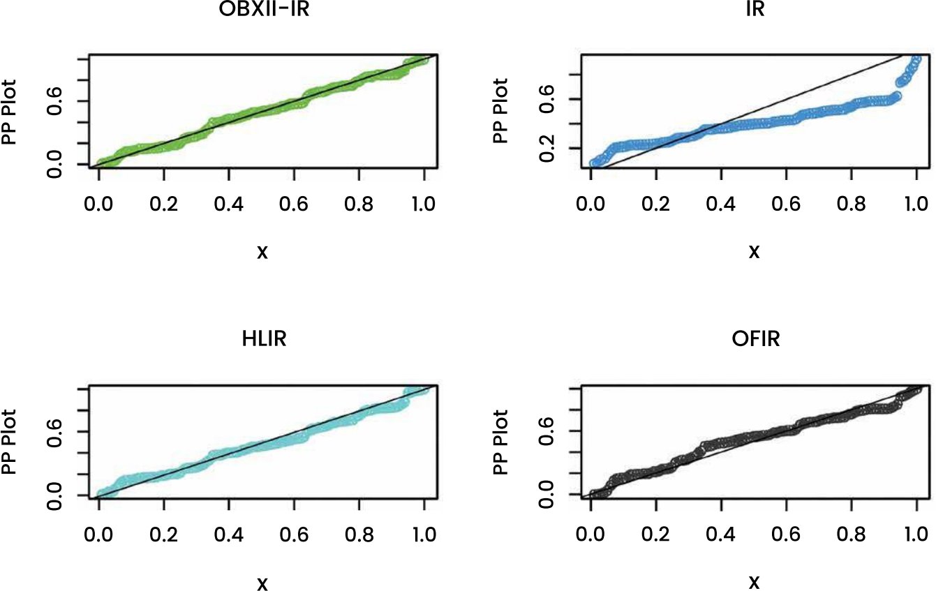
To enhance the numerical results listed in Tables 8 and 9, the model fit quality was graphically represented across (Fig. 7–9) using real experimental data for carbon fibers, and the geometric reading of these drawings shows the following:

Fig. (7). Graphical comparison of pdf for different models with the experimental distribution of data.

Fig. (8). Graphical comparison of the cdf for different models.

Fig. (9). Shows the P–P Plot for the OBXII-IRD and the comparative models, to show how well the proposed distribution matches the data.

Fig. (7) shows the pdf plotted for the various distributions overlaid on the bar graph (histogram) of the actual experimental data distribution. It is observed that the OBXII-IRD curve (represented by its corresponding color) is the only distribution that correctly tracks the rise and fall of the bar graphs, covering the distribution peak with exceptional accuracy and providing a flexible fit to the rightward skew of the data.

Fig. (8) depicts the cdf for the OBXII-IRD and the comparative distributions. A high degree of geometric agreement is noticed between the OBXII-IRD curve and the data curve. This agreement decressed progressively for the IR, OFIR, and HLIR distributions, which explains why the proposed distribution achieved the lowest KS statistic value.

Fig. (9) presents the p-p plot considered one of the accurate tools for assessing goodness of fit, which illustrates the relationship between the cumulative probabilities and its theoretical counterpart. The figure clearly demonstrates the probability points for the OBXII-IRD constant matching with the reference line. This shows a lack of dispersion or deviation, therefore presenting that the OBXII-IRD is more efficient than the other distributions.

CONCLUSION

This study provided an in-depth analysis of the efficiency of different estimation methods for the OBXII-IRD, where the results showed the consistency of all estimation methods, with the estimated values converging from the true values of the parameters as the sample size increased, while the probability of coverage (CP) remained stable. As for the comparison between non-Bayesian methods, the KE method has consistently proven its superiority, followed by the MLE method.

Regarding entropy measures, seven distinct entropy measures were derived and analyzed to assess the degree of uncertainty associated with the OBXII-IRD. The Reny entropy measure proved to be the most effective at representing the behavior of the OBXII-IRD compared to the other measures. The analysis revealed that increasing the values of the parameters resulted in lower entropy values, indicating reduced uncertainty. Conversely, increasing the value of the parameter led to a higher level of dispersion. A practical application using carbon fiber data analyzed via the MLE demonstrated that the OBXII-IRD provided a better fit than IR, HLIR, and OFIR distributions, a conclusion supported by a p-value of 0.8668.

LIST OF ABBREVIATIONS

ACI	=	Approximate Confidence Interval
KE	=	Kolmogorov Estimation
MLE	=	Maximum Likelihood Estimation
MPS	=	Maximum Product space Estimation
OBXII-IRD	=	Odd Burr Inverse Rayleigh

AUTHORS’ CONTRIBUTION

A.A.K. contributed to the study concept and design and writing of the paper. M.A.K. contributed to the study concept and design and writing of the paper. A.M.S. contributed to data collection and writing of the paper. A.T.M. contributed to data collection, review, and editing. Q.N.H. contributed to data analysis or interpretation, review, and editing. M.K.A.H. contributed to data analysis or interpretation, review, and editing. All authors reviewed and approved the final version of the manuscript.

ETHICAL APPROVAL & INFORMED CONSENT

The following study does not involve any human participants, clinical trials, or animal tests. Moreover, ethical approval and informed consent were not required for this research. Section 6 represents previously published physical measurements of carbon fiber materials science tensile strength, which are publicly available.

AVAILABILITY OF DATA AND MATERIALS

The data used in this study are publicly available and were obtained from previously published sources. The dataset analyzed in this work is cited appropriately in the manuscript. The simulation results and computational procedures can be reproduced using the methods and details provided in the article.

FUNDING

This research received no financial support from any public, commercial, or not-for-profit funding agency.

CONFLICT OF INTEREST

The authors declare that they have no competing interests that may influence this study.

ACKNOWLEDGEMENTS

None.

DECLARATION OF AI

The authors declare that this research project did not use any artificial intelligence tools or technologies in the process of preparing, analyzing, or writing the study and the authors take full responsibility for the content and originality of this work.

REFERENCES

[1]Treyer VN. Inverse Rayleigh (IR) model. Proc. USSR Acad. Sci. 1964.

[2] Voda VG. On the inverse Rayleigh distributed random variable. Rep Statis App Res JUSE. 1972;19(4):13–21.

[3] Gharraph MK. Comparison of estimators of location measures of an inverse Rayleigh distribution. Egypt Stat J. 1993; 37(2): 295–309.
https://doi.org/10.21608/esju.1993.426926

[4] Howlader HA, Hossain AM, Makhnin O. Bayesian prediction bounds for Rayleigh and inverse Rayleigh lifetime models. J Appl Stat Sci. 2009; 17(1).
https://doi.org/10.47013/19.2.3

[5] Banerjee P, Bhunia S. Exponential Transformed Inverse Rayleigh distribution: Statistical properties and different methods of estimation. Austrian J Stat. 2022; 51(4): 60–75.
http://dx.doi.org/10.17713/ajs.v51i4.1338

[6] Khan MS, King R. Transmuted modified Inverse Rayleigh distribution. Austrian J Stat. 2015; 44(3): 17–29.
https://doi.org/10.17713/ajs.v44i3.21

[7] Goual H, Yousof HM. Validation of Burr XII inverse Rayleigh model via a modified chi-squared goodness-of-fit test. J Appl Stat. 2020; 47(3): 393–423.
https://doi.org/10.1080/02664763.2019.1639642

[8] Cordeiro GM, Yousof HM, Ramires TG, Ortega EMM. The Burr XII System of densities: properties, regression model and applications. J Stat Comput Simul. 2018;88(3):432–456.
https://doi.org/10.1080/00949655.2017.1392524

[9] Ali S. Mixture of the inverse Rayleigh distribution: Properties and estimation in a Bayesian framework. Appl Math Model. 2015; 39(2): 515–530.
http://dx.doi.org/10.1016/j.apm.2014.05.039

[10] Fisher RA. The effect of methods of ascertainment upon the estimation of frequencies. Ann Eugen. 1934; 6(1): 13–25.
https://doi.org/10.1111/j.1469-1809.1934.tb02105

[11] Rao CR. On discrete distributions arising out of methods of ascertainment. Sankhyā: Indian J Stat Ser A. 1965; 27: 311–324.
https://www.jstor.org/stable/25049375

[12] Aydın D. The new weighted inverse Rayleigh distribution and its application. Facta Univ Ser Math Inform. 2019; 34(3): 511-523.
https://doi.org/10.22190/FUMI1903511A

[13] Rao GS, Mbwambo S. Exponentiated inverse Rayleigh distribution and an application to coating weights of iron sheets data. J Probab Stat. 2019; 2019: 1–13.
https://doi.org/10.1155/2019/7519429

[14] Kamnge JS, Chacko M. Half logistic exponentiated inverse Rayleigh distribution: Properties and application to life time data. PLoS One. 2025; 20(1): e0310681.
https://doi.org/10.1371/journal.pone.0310681

[15] Yanuar F, Iqbal M, Devianto D, Zetra A, Asdi Y, Ilahi R, & Sani, RF. Bayesian estimation under different loss functions for the case of inverse Rayleigh distribution. Kuwait J Sci. 2025; 52(1): 100343.
https://doi.org/10.1016/j.kjs.2024.100343

[16] Asif M, Raftab M, Usman M, Khan AA. Analysis of parameters of the exponentiated inverse Rayleigh distribution under the Bayesian framework. Kuwait J Sci. 2025; 52(3): 100424.
https://doi.org/10.1016/j.kjs.2025.100424

[17] Alghamdi AS. Marshall-Olkin Exponentiated Inverse Rayleigh Distribution Using Bayesian and Non-Bayesian Estimation Methods. Symmetry. 2025; 17(5): 707.
https://doi.org/10.3390/sym17050707

[18] Cover TM, Thomas JA. Elements of Information Theory. 2nd ed. New York: John Wiley & Sons; 2006.
https://doi.org/10.1002/047174882X

[19] Shannon CE. A mathematical theory of communication. Bell Syst Tech J. 1948; 27(3): 379–423.
https://doi.org/10.1002/j.1538-7305.1948.tb01338.x

[20] Rényi A. On measures of entropy and information. In: Proceedings of the Fourth Berkeley Symposium on Mathematical Statistics and Probability. 1960; 1: 547–61. Available From: https://www.scirp.org/reference/referencespapers?referenceid=2095576

[21] Tsallis C. Possible generalization of Boltzmann-Gibbs statistics. J Stat Phys. 1988; 52(1–2): 479–87.
http://dx.doi.org/10.1007/bf01016429

[22] Arimoto S. Information-theoretical considerations on estimation problems. Inf Contr. 1971; 19(3): 181–94.
http://dx.doi.org/10.1016/s0019-9958(71)90065-9

[23] Havrda J, Charvát F. Quantification method of classification processes. Concept of structural a-entropy. Kybernetika. 1967; 3(1): 30–5.
http://dml.cz/dmlcz/125526

[24] Gupta HC, Sharma BD. On non-additive measures of inaccuracy. Czechoslov Math J. 1976; 26(4): 584–95.
http://dx.doi.org/10.21136/CMJ.1976.101429

[25] Sant’Anna AP, Taneja IJ. Trigonometric entropies, Jensen difference divergence measures, and error bounds. Inf Sci. 1985; 35(2): 145–56.
https://doi.org/10.1016/0020-0255(85)90046-5

[26] Khalaf AA, Khaleel MA, Jawa TM, Sayed-Ahmed N, Tolba AH. A Novel Extension of the Inverse Rayleigh Distribution: Theory, Simulation, and Real-World Application. Appl Math Inf Sci. 2025; 19(2): 467–488.
http://dx.doi.org/10.18576/amis/190220

[27] Khalaf AA, El-Saeed AR, Khaleel MA, Tolba AH. The four-parameter odd generalized Rayleigh Lomax distribution: Theory, simulation, and applications. Symmetry. 2026; 18(2): 244.
http://dx.doi.org/10.3390/sym18020244

[28] Abdulqader Salih S, Mahmood Ali D, Khaled Kolaib H, Abdulrahman Khalaf A. Truncated Exponentiated Ailamujia Exponential distribution: Properties and applications. Baghdad Sci J. 2026; 23(1): 271–90. Available from: http://dx.doi.org/10.21123/2411-7986.5183

[29] Khalaf AA, Haleel MA. The new strange Generalized Rayleigh family: Characteristics and applications to COVID-19 data. Iraqi J Comput Sci Math. 2024; 5(3).
http://dx.doi.org/10.52866/ijcsm.2024.05.03.005

[30] Khalaf AA, Khaleel MA. The Odd Burr XII Exponential distribution: Properties and applications. In: AIP Conference Proceedings. 2025; 3264(1).
https://doi.org/10.1063/5.0258451

[31] Khalaf AA, Khaleel MA, Tolba AH, Ahmed NS. Classical Inference for the Five Parameter Exponentiated Weibull Distribution: Properties and Applications in Health and Reliability. 2025; 14: 469–492.
http://dx.doi.org/10.18576/jsap/140310

[32] Gemeay A M, Sapkota L P, Tashkandy Y A, Bakr M E, Balogun OS, Hussam E. New bounded probability model: Properties, estimation, and applications. Heliyon. 2024; 10 (23).‏
https://doi.org/10.1016/j.heliyon.2024.e38965

[33] Leão J, Saulo H, Bourguignon M, Cintra RJ, Rêgo LC, Cordeiro GM. On some properties of the beta inverse Rayleigh distribution. arXiv. 2022.
http://arxiv.org/abs/2206.01229

[34] Almarashi AM, Badr MM, Elgarhy M, Jamal F, Chesneau C. Statistical inference of the half-logistic inverse Rayleigh distribution. Entropy. 2020; 22(4): 449.
http://dx.doi.org/10.3390/e22040449

[35] Elgarhy M, Alrajhi S. The odd Fréchet inverse Rayleigh distribution: statistical properties and applications. J Nonlinear Sci Appl. 2018; 12(5): 291–299.
http://dx.doi.org/10.22436/jnsa.012.05.03

[36] Nichols MD, Padgett WJ. A bootstrap control chart for Weibull percentiles. Quality and reliability engineering international. 2006; 22: 141–51.
https://doi.org/10.1002/qre.691