
pdpublishers.com

Article ID: PD2601208007

Views: 653
Volume 1 (2026)
Published 04 Sep 2026

Forecasting Inflation with Machine Learning and Traditional Time-Series Models: A Multi-Horizon Rolling-Origin Assessment

📚 Cited by: 0

⬇ Downloads: 38


Author

1COMSATS Institute of Information and Technology Lahore, Lahore, Pakistan

Article History:

Received: 08 June, 2026

Accepted: 29 August, 2026

Revised: 28 August, 2026

Published: 04 September, 2026

ABSTRACT:

Introduction: The role of inflation forecasting in the monetary-policy assessment, financial planning and macroeconomic decision-making is crucial. This study also compares the Seasonal Autoregressive Integrated Moving Average (SARIMA) and Extreme Gradient Boosting (XGBoost) models to forecast Sticky Price Consumer Price Index (Sticky CPI) in the United States of America (USA) for seasonality during the past decade.

Methodology: The current-vintage dataset (January 1968 to August 2024) contains 680 observations. All the 200 test months (Jan. 2008-Aug. 2024) were set aside for pseudo-out-of-sample evaluation, while the rest of the months (Jan. 1968-Dec. 2007) were used for model development only. One SARIMA order was selected one time from the pre-2008 sample and then these coefficients were re-estimated at each forecast origin. Recursive forecasts were obtained from a single SARIMA specification. XGBoost was fine-tuned separately for each horizon using five validation folds with a growing window that were completely nested within the pre-2008-time frame, with the hyperparameters fixed and the corresponding direct models re-estimated at each origin.

Results: The reproduced analysis does not hold true for the 12-month XGBoost advantage. SARIMA records the lowest RMSE at all four horizons: 0.0869, 0.2420, 0.4229 and 0.9611, compared with XGBoost values of 0.1940, 0.4314, 0.7564 and 1.3040. After Holm adjustment, SARIMA is favored by Harvey-Leybourne-Newbold corrected Diebold-Mariano tests at 1, 3 and 6 months compared to XGBoost, while it is not significant at 12 month (p = 0.0673). Under a moving-block bootstrap, the 12-month RMSE is significantly larger for the predefined post-2020 analysis for all models, with SARIMA having a much smaller RMSE than XGBoost during that time. Additionally, feature ablation indicates that the entire nonlinear specification of XGBoost is weaker than a linear ridge model with the same features, after regularisation. Prediction intervals are conservative for both types of models, and SARIMA intervals are narrower and have lower interval scores.

Conclusion: The results provide support to the discipline of benchmark evaluation, uncertainty reporting and monitoring of model-combination superiority through machine-learning, but do not support unconditional superiority of machine-learning.

Keywords: Inflation forecasting, sticky CPI, SARIMA, XGBoost, rolling-origin evaluation, direct forecasting, recursive forecasting, forecast uncertainty.

1. INTRODUCTION

Inflation forecasting is a central problem in applied macroeconomics because expected inflation influences monetary policy decisions, financial market valuation, wage bargaining, contract design and household planning [1, 2]. Forecasting inflation is nevertheless difficult because inflation combines persistent serial dependence with episodes of rapid change. Recent inflation values often contain useful information for short-horizon forecasts, but supply disturbances, changes in demand, monetary-policy responses and shifts in expectations can alter the inflation path over longer horizons [3].

One of the most important empirical properties of inflation is persistence. Sticky price adjustment, wage-setting arrangements, adaptive expectations and delayed policy transmission can cause inflation to respond gradually to disturbances [46]. This persistence allows autoregressive and naive forecasts to remain competitive, particularly at short horizons. However, a stable autoregressive relationship cannot represent every inflation episode. The post-2020 increase in US inflation combined supply constraints, relative-price changes, labour-market pressures and demand-related influences that were difficult to anticipate using lagged inflation alone [710].

These properties have different approaches to them across classical time-series and machine-learning models. SARIMA accounts for linear auto-regression, moving-average and seasonal relationship in an economical model or stochastic model [1113]. XGBoost has the ability to model nonlinear decision-tree partitions, and can model conditional relationships between lagged values and rolling statistics [1417]. More flexibility could be of benefit in case the relation turns out to be nonlinear, but also adds sensitivity to the choice of the hyper-parameters and can make overfitting more likely when samples are relatively small, as is common with macro-economic data.

The prediction horizon also affects the accuracy of forecasts. The forecast for one month of inflation is sensitive to the most recent inflation figure, and a 12 months forecast would have higher levels of accumulated uncertainty. Measures of how well one-step-ahead forecasts are realized may therefore be misleading if used to assess comparative performance. The leakages were studied at 1-, 3-, 6- and 12-month time horizons for some common target dates in a leakage-controlled rolling-origin design.

RQ1: How do SARIMA, XGBoost, naive and seasonal-naive forecasts compare at 1-, 3-, 6- and 12-month horizons?

RQ2: Does relative performance differ between predefined pre-2020 and post-2020 target periods?

RQ3: Are pairwise loss differences statistically significant after accounting for overlapping multi-step errors and multiple testing?

RQ4: Which XGBoost feature groups contribute to their forecast performance?

RQ5: How well calibrated and sharp are the models’ 80% and 95% prediction intervals?

H1: The relative predictive performance of SARIMA and XGBoost is horizon dependent, with SARIMA expected to perform strongly at shorter horizons and XGBoost potentially improving relative to SARIMA at the 12-month horizon.

H1 is evaluated using changing error rankings and horizon-specific pairwise comparisons. It is not treated as though one omnibus test directly establishes horizon dependence. The reproduced evidence ultimately does not support the hypothesised ranking reversal because SARIMA records the lowest RMSE on every horizon.

The contribution is not the first one that uses XGBoost for inflation forecasting (which is already established). Rather, in this study the univariate re-evaluation is done under the controlled setting of SARIMA and the XGBoost model share the same Sticky CPI history. It blends the advantages of pre-specified models, of separating and directly specifying the recursive and direct strategies, of common dates of forecast, of naive benchmarks, of forecast accuracy tests, of prediction intervals, of a predetermined period comparison, of feature ablation and of prediction combination. The design thus focuses on the replicability of the findings, and minimizes the risk that differences are caused by differential access to external macroeconomic predictors.

2. LITERATURE REVIEW

2.1. General Forecasting and Economic Time-Series Evaluation

A forecasting experiment is reliable if it maintains the order of the information as it arrives. Later observations can be used for model development for earlier forecasts by random cross validation. Instead, the rolling-origin and expanding-window procedures sequentially step the origin and use only information up to the current origin to form each prediction [18]. This results in repeating out-of-sample errors and is not reliant on any one arbitrary hold out date.

Multi-step forecasts can be recursive or non-recursive. A recursive strategy estimates one model and then extends it out to longer time horizons, and may build up errors. A direct strategy is the estimation of a distinct model for each horizon, with no attempt to use shorter-horizon predictions in the following steps, at the cost of having more models. The differences in the performance can thus be attributed to both the model family and multi-step strategy [19, 20].

Clear standards are a must. A naive forecast is used to check if the sophisticated model is better than the persistence model; a seasonal-naive model is used to check annual repetition. The consensus evidence is the lower value of RMSE or MAE, but formal comparison of forecasts needs a loss-differential test. The errors in multi-step forecasts may be serially correlated, which can justify the use of HAC variance estimation and finite-sample [21, 22].

Forecasts of point values are also inadequate when considering policy applications. Empirical coverage, width and proper scoring rules need to be used to evaluate prediction intervals [23, 24]. Model selection risk can be minimized by forecasting combinations, though the importance of assessing combinations out of sample is not emphasized [25].

2.2. Inflation Persistence and Forecasting

The persistence of inflation reflects the persistence of a relation with the inflation’s past and the gradual response to inflation changes. It may be due to delayed policy transmission, expectations, wage-setting mechanisms and price stickiness [3, 26]. Statistically, persistence appears through positive autocorrelation over several lags.

Although AR methods are increasingly employed for preventing this problem, ARIMA type models are still widely applied in this area because they make apparent serial dependence and provide uncertainty estimates of the model. Their limitations occur when there is change in linear relationships or when recycled errors occur [27]. Machine learning methods give regularisation and non-linear function approximation; however, some benefits from their use rely on the information content, on the number of samples and on the design of the validation [28, 29].

No literature supports universal machine-learning superiority. In data-rich settings, flexible models can be useful, while simpler autoregressive models can be easily outperformed by inflation’s high persistence [30]. A controlled univariate design is then useful to assess whether the addition of value to the series into nonlinear feature transformations is worth the added model complexity when the same series is used for both model families.

2.3. Predefined Period Analysis

The differences in inflation levels and volatility can be easily seen among the 70s, the Great Moderation, and the post-2020 episode [29, 30]. The post-2020 inflation episode is thus regarded as a helpful ad hoc stress scenario as it represented both supply-side restrictions, price shocks, labour-market pressures and inflation expectations. Recent studies on pandemic-era inflation have highlighted how these forces affected the short-run inflation environment, and the challenge of forecasting inflation. In the broader literature, formal methods of structural breaks are appropriate, but are not employed to pinpoint a break date in this research. The a priori target-date split for January-2020 is solely for showing performance for that point in time. In line with this, the analysis below considers only the specified periods, the pre-2020 inflation episode and episode of increased instability; it does not suggest that a breakpoint is actually found here, but simply background details and future extensions are mentioned.

2.4. Research Gap

Although inflation forecasting has been extensively examined using traditional econometric models and, more recently, machine-learning methods, several methodological gaps remain. First, many machine-learning studies use data-rich predictor sets containing labour-market, financial, monetary, commodity-price and expectations variables. Such studies demonstrate the potential value of flexible algorithms but do not isolate whether improvements arise from the nonlinear model itself or from access to a larger information set. There is, therefore a need for a controlled comparison in which classical and machine-learning models receive the same underlying historical information.

Second, existing studies frequently concentrate on one-step-ahead or a limited number of forecast horizons. This provides an incomplete assessment because the persistence, uncertainty and information requirements of inflation forecasting change as the horizon increases [31, 32]. Moreover, comparisons between statistical and machine-learning approaches do not always clarify whether multi-step predictions are generated recursively or through separate direct models. Since recursive and direct strategies have different bias–variance properties, failing to distinguish them can obscure the source of observed performance differences.

Third, the temporal validation procedures used in machine-learning forecasting are not always reported with sufficient precision. Studies can use a general reference of rolling or expanding validation, even if the actual training dates are not mentioned, the number of validation folds is not mentioned, the sample size is not mentioned for the different horizons and the hyperparameters are not re tuned during the final evaluation. This raises questions on how repeatable the results are and the chance of introducing look-ahead bias. Multi-step forecast errors have also to be treated appropriately for overlapping (finite-sample, treatment of multiple forecast comparisons) but the loss differential direction is not always reported.

The fourth, the comparative literature is focused on providing point forecast accuracy, and less on providing prediction-interval coverage, interval width, feature-group contribution and forecast combinations. As a result, it is difficult to distinguish between a model that has a low average error and one that has well-calibrated uncertainty estimates – and whether the success of a model is due to lagged or rolling predictors. Another typical type of interpretation of period-specific evaluations is as evidence of structural change, without making a formal breakpoint estimate.

This paper strives to fill these gaps by conducting a univariate and multi-horizon controlled comparison of SARIMA and XGBoost based on same history of the Sticky CPI. It uses an explicit model specified separately for the development set, a set of 5 validation folds of the expanding window choosing the target dates for each explicitly provided, deterministic model choices, recursive SARIMA models (may be used for the top level forecasting model), direct XGBoost models for the forecasts within a given window (expanding window across the folds) and a common set of target dates for the out-of-the-sample forecasts. The comparison also includes a number of naive benchmarks, tests of forecast error, prediction intervals, feature-group ablation and forecast combinations as well as a clearly defined pre-2020/post-2020 period analysis. The trick here is the transparency of the methodology, and the ability to reproduce and develop meaningful comparisons rather than ascribing the first use of machine learning to inflation forecasting.

3. METHODOLOGY

3.1. Empirical Pipeline

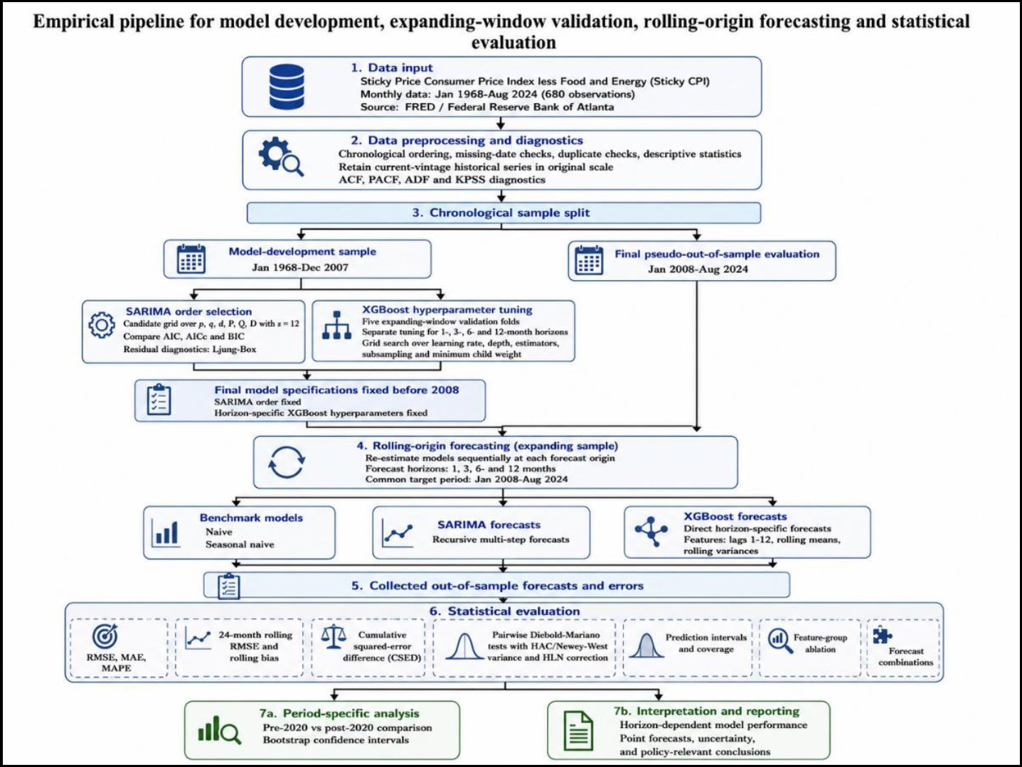
The design is summarised in Fig. (1). The pre-2008 sample is employed for diagnostic analysis, order selection with SARIMA model and tuning for XGBoost across horizons. The 200 target months used for the last pseudo out-of-choice test is the same for all the horizons. The difference lies in the orders for both the SARIMA and the four separately tuned direct horizon-specific models of XGBoost: the SARIMA has a fixed order and creates recursive multi-step forecasts, while XGBoost has four different orders and creates four independently tuned direct horizon-specific forecasts. Point accuracy, interval performance and pairwise forecast-accuracy tests or predefined-period comparisons, feature ablations and combinations of forecasts are subsequently assessed.

Fig. (1). Empirical pipeline for model development, expanding-window validation, rolling-origin forecasting and statistical evaluation.

3.2. Dataset

This study is based on the Sticky Price Consumer Price Index Less Food and Energy (Sticky CPI) series, CORESTICKM159SFRBATL, available from the Federal Reserve Bank of Atlanta and from Federal Reserve Economic Data (FRED) [6, 26]. The series is published monthly, seasonally adjusted and as a percentage change from 12 months earlier. The current-vintage sample includes 680 observations for the period January 1968 to August 2024. The mean it has reproduced is 4.331%, with a sample standard deviation of 2.684 percentage points, a minimum of 0.664% and a maximum of 15.774% (Table 1).

Table 1. Dataset description and descriptive statistics.

ItemDescription/value
Formal Series NameSticky Price Consumer Price Index Less Food and Energy
AbbreviationSticky CPI
Series CodeCORESTICKM159SFRBATL
SourceFRED / Federal Reserve Bank of Atlanta
FrequencyMonthly
UnitsPercent change from year ago, seasonally adjusted
PeriodJanuary 1968-August 2024
Observations680
Mean4.331%
Standard Deviation2.684 percentage points
Minimum0.664%
Maximum15.774%

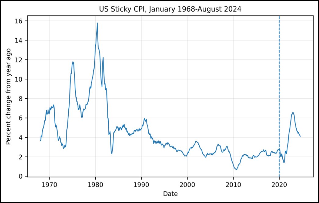
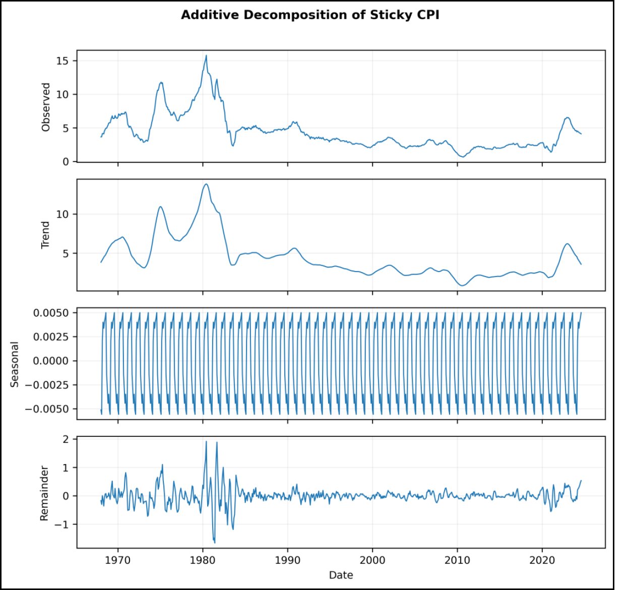
The inflation rate has experienced significant changes over time, particularly during the 1980s and again following 2020, as seen in Figs. (2 and 3). The additive decomposition suggests significant long-run trends, a very small seasonal variation compared to the trend, and higher irregular deviations in periods of high inflation turmoil.

Fig. (2). US sticky CPI from january 1968 to august 2024.

Fig. (3). Additive trend, seasonal and remainder components of sticky CPI.

3.3. Preprocessing and Temporal Validation

The dates were adjusted to a monthly scale, and anomalies were identified and removed using a time series analysis with a complete time series from January 1968 to August 2024. There have been no “holes” in the series, no double dates, or non-numeric data. Various inflation observations for this series were more meaningful on an economic basis, and were therefore retained, rather than winsorised. No scaling applied, SARIMA is estimated on the proportion scale (from 0 to 100) and XGBoost is also on the same level due to the distance-based standardisation of tree partitions not being a prerequisite requirement. All lagged and/or rolling features were moved to be contained within the feature vector at origin timestep t only. The model development took place between January 1968 until December 2007. The last evaluation period was the same 200 planning targets between January 2008 and August 2024; for target T and horizon h, the period between T and T-h months was used for the planning period of forecast Origin. This common target design ensures that comparisons between different areas of the sky are relevant and that different samples are not involved.

3.3.1. Stationarity Assessment

The development sample used prior to 2008 was used for estimates of the ADF and KPSS tests. The level series is not rejected as a unit root when the constant-only ADF is used (p = 0.0817), but is rejected at 5% when the level ADF is specified with the trend (p = 0.0188), revealing sensitivity to the deterministic specification of the ADF. The first difference of the consumer price index also fails to show a unit root either in the constant-only specification (p = 0.0006) or in the constant-plus-trend specification (p = 0.0045). KPSS does not reject stationarity as originally observed (p = 0.010), but rejects stationarity as first difference (p > 0.100). A choice was made to use d = 1 as first differencing provides concordant evidence both in these test families and in the deterministic specifications. This decision is not based on the level ADF result obtained from just one trend indicator (Tables 2 and 3).

Table 2. Augmented dickey-fuller stationarity tests.

SeriesSpecificationLagsStatisticp-value1% CV5% CV10% CV
LevelConstant18-2.65750.0817-3.4446-2.8678-2.5701
LevelConstant + trend18-3.75780.0188-3.9785-3.4201-3.1327
First differenceConstant17-4.20880.0006-3.4446-2.8678-2.5701
First differenceConstant + trend17-4.19860.0045-3.9785-3.4201-3.1327

Table 3. KPSS stationarity tests.

SeriesSpecificationLagsStatisticp-value
LevelConstant121.79690.010
LevelConstant + trend120.22840.010
First differenceConstant90.078>=0.100
First differenceConstant + trend90.0505>=0.100

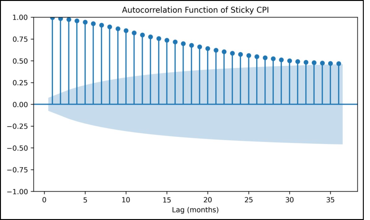
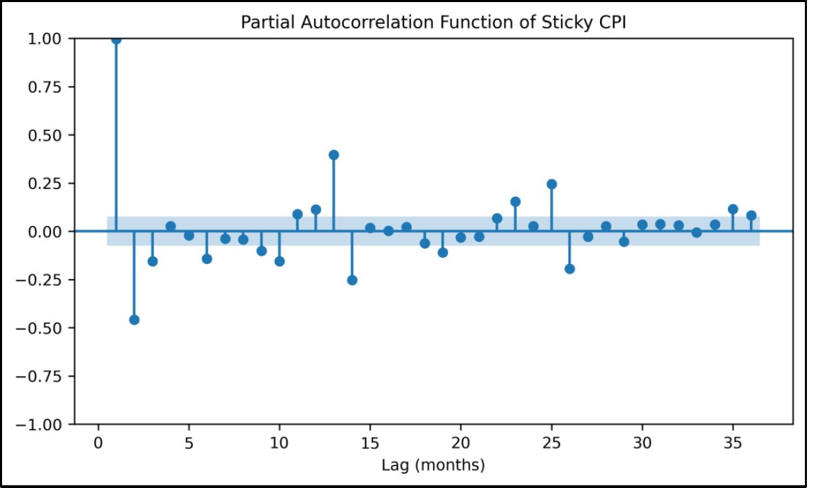
Noisy ACF suggests high and sustained correlation of serial changes. There is a significant first lag feature in the PACF along with a few other big lags (Figs. 4 and 5). The plots are included simply as diagnostic plots as evidence of recent persistence was insufficient for the final order of the SARIMA.

Fig. (4). Autocorrelation function of Sticky CPI.

Fig. (5). Partial autocorrelation function of Sticky CPI.

3.4. Five Expanding-Window Validation Folds

For each horizon, the tuning of XGBoost was conducted independently and a fifth subset of four years was used for validation, all contained in the past. The 240 validation forecasts were equally split between each of the 48 months in each of the two folds. Training was performed on a one-month increment at each origin with only feature-target pairs for which the target had been observed (Tables 4 and 5).

Table 4. Expanding-window validation dates.

FoldTarget Dates1-Month Origins3-Month Origins6-Month Origins12-Month OriginsValidation n
11988-01 to 1991-121987-12 to 1991-111987-10 to 1991-091987-07 to 1991-061987-01 to 1990-1248
21992-01 to 1995-121991-12 to 1995-111991-10 to 1995-091991-07 to 1995-061991-01 to 1994-1248
31996-01 to 1999-121995-12 to 1999-111995-10 to 1999-091995-07 to 1999-061995-01 to 1998-1248
42000-01 to 2003-121999-12 to 2003-111999-10 to 2003-091999-07 to 2003-061999-01 to 2002-1248
52004-01 to 2007-122003-12 to 2007-112003-10 to 2007-092003-07 to 2007-062003-01 to 2006-1248

Table 5. Usable training pairs at the first origin of each fold.

Foldh = 1h = 3h = 6h = 12Validation Targets
122822421820648
227627226625448
332432031430248
437236836235048
542041641039848

3.5. Forecasting Strategies and Benchmarks

SARIMA uses one order for all horizons. The order was selected once from January 1968-December 2007, fixed thereafter, and its coefficients were re-estimated at every forecast origin. Forecasts at 1, 3, 6 and 12 months were generated recursively from this single specification. XGBoost uses a direct strategy: separate supervised targets y (t+1), y (t+3), y (t+6) and y (t+12) were trained and tuned independently, and shorter-horizon predictions were not inputs to longer-horizon predictions. The comparison should therefore be interpreted as a comparison of complete forecasting systems – recursive SARIMA versus direct horizon-specific XGBoost – rather than as a pure algorithmic comparison in which the multi-step strategy is held constant. The naive forecast is a forecast based on the value at the forecast origin, and the forecast value using the seasonal naive approach equals the observed value for the same target month 1 year earlier. These two benchmark definitions are equivalent at the 12-month time horizon because the origin is set 12 months before the target.

3.6. SARIMA Selection and Diagnostics

The candidate grid spanned a range of P and Q from 0-2, of d 0-1, of seasonal P and D 0-1, and for s = 12, resulting in 144 specifications. The sample prior to 2008 was used to infer candidate models and the ranking was based on AIC, AICc and BIC. The lowest-AIC specification was SARIMA (2,1,1) (1,0,1) [12], with AIC -206.829, AICc -206.652 and BIC -181.977.

Residuals for white-noise (given the selected model) are not shown in the reproduced diagnostics. Ljung-Box tests give Q (12) = 21.001 (p = 0.0038) and Q (24) = 48.184 (p = 0.0002), so statistically significant residual autocorrelation remains. Residual independence belongs to the vital adequacy diagnostics of SARIMA-related analyses, and is of particular importance for uncertainty calculations using models. The model is still used and not selected again after the final evaluation results, but it ended up being the lowest AIC (desired model). The non-independence of the remaining autocorrelation however will not vitiate the comparative pseudo-out of sample error analysis, as in all comparative tests used, the same targets are being used to test all models and the loss inference used is conducted on HAC-adjusted tests that allow for serial correlation in the forecasts’ loss difference. It does, however, signal less-than-perfect specification of SARIMA, and will be declared as a special case, especially in the context of the model-based prediction intervals in Table 6.

Table 6. Ten leading SARIMA candidates from the pre-2008 sample.

ModelAICDelta AICAICcBICQ(12), pQ(24), p
SARIMA(2,1,1)(1,0,1)[12]-206.8290.000-206.652-181.97721.001 (0.0038)48.184 (0.0002)
SARIMA(2,1,2)(1,0,1)[12]-203.9762.853-203.739-174.99719.678 (0.0032)46.472 (0.0003)
SARIMA(2,1,1)(0,0,1)[12]-203.6093.220-203.483-182.89926.358 (0.0009)55.121 (0.0000)
SARIMA(1,1,2)(1,0,1)[12]-201.3335.496-201.155-176.49427.421 (0.0003)55.030 (0.0000)
SARIMA(2,1,2)(0,0,1)[12]-201.0325.797-200.854-176.19324.074 (0.0011)52.520 (0.0001)
SARIMA(1,1,2)(0,0,1)[12]-198.2908.539-198.163-177.59133.166 (0.0001)62.851 (0.0000)
SARIMA(1,1,1)(1,0,1)[12]-193.26513.564-193.138-172.55536.640 (0.0000)67.669 (0.0000)
SARIMA(1,1,1)(0,0,1)[12]-191.16515.664-191.081-174.59741.108 (0.0000)73.664 (0.0000)
SARIMA(2,1,0)(0,0,1)[12]-182.74224.087-182.658-166.16629.615 (0.0005)62.060 (0.0000)
SARIMA(2,1,0)(1,0,1)[12]-182.66724.162-182.540-161.95726.324 (0.0009)56.708 (0.0000)

3.7. XGBoost Model and Hyperparameter Selection

The direct XGBoost predictors were lags 1-12, rolling means over 3, 6 and 12 months and rolling variances over the same windows. The grid contained 144 transparent candidate combinations per horizon: learning rate {0.03, 0.10}; maximum depth {2, 3, 5}; estimators {100, 200, 300}; subsample {0.8, 1.0}; column subsample {0.8, 1.0}; and minimum child weight {1, 3}. The seed used was 42 for a fixed seed.

Tuning was done once prior to January 2008, and then separately to each forecast horizon. The chosen hyperparameters for the XGBoost model were then kept constant for the subsequent evaluation and the horizon model was re-estimated as the rolling origin moved to the right. Separating information in order that information not used in the final period do not impact on information that is used to select the model, as well as explicitly showing the direct forecasting strategy (Tables 7 and 8).

Table 7. Horizon-specific XGBoost settings.

Parameter1 Month3 Months6 Months12 Months
Learning Rate0.030.030.030.03
Maximum Depth2333
Estimators300200200100
Subsample0.81.00.81.0
Column Subsample1.00.81.00.8
Minimum Child Weight3131
Mean Validation RMSE0.27160.61411.09052.0430

Table 8. Validation RMSE by fold and horizon.

Fold1 Month3 Months6 Months12 Months
10.18950.42630.61110.5929
20.24940.44971.08272.3284
30.67701.54652.62505.0709
40.13630.40650.66981.2330
50.10560.24160.46410.9899
Mean0.27160.61411.09052.0430

3.8. Accuracy, Statistical Testing and Uncertainty

Standard accuracy measures such as RMSE, MAE and MAPE [10] were used to assess the point accuracy. The primary reason for considering the RMSE and MAE is that percentage errors can be unstable at low levels of inflation. Bias is the difference between actual and forecasted (actual – forecast) and negative bias corresponds to over-prediction while positive bias corresponds to under-prediction.

The squared error loss function and the DM test are used in pairwise comparisons. The loss differential, defined as d(t) = e_A(t)^2 – e_B(t)^2, would then be less to the benefit of model A. For multi-step errors the second, long-run variance is estimated using a Newey-West HAC estimator with lag h-1 [22]. A finite sample correction of Harvey-Leybourne-Newbold is used, and p-values are two-sided [21]. Holm adjustments are provided both overall across all 12 pairwise tests, and within each family of comparisons across the four horizons.

(1)

SARIMA intervals are model-based. XGBoost intervals use symmetric empirical absolute-error quantiles calibrated from the 240 pre-2008 validation forecasts at each horizon. Interval performance is evaluated using empirical coverage, mean width and mean interval score. The SARIMA intervals are model based. Split intervals for XGBoost are computed as the symmetric empirical absolute-error quantiles based on 240 pre-2008 forecast ensemble validation data for each horizon. The empirical coverage, the mean width and interval score [23, 24] can be used to assess interval performance. Since those XGBoost intervals are customarily called validation-calibrated empirical intervals, rather than finite-sample conformal guarantees that hold in independent samples, it warrants additional consistencies in the descriptions. The predefined 12 months comparison period uncertainty in RMSE and difference in RMSE between two models (between RMSE of RMSEs), were computed using a moving-block bootstrap to the aligned forecast-error pairs within each period. A 12-month block length, 3,000 bootstrap replications and the fixed random seed of 42 were used. The model alignment and local serial dependence between underlying model errors are preserved as reported 95% percentile (or bootstrap) confidence intervals: those intervals defined by the empirical 2.5th and 97.5th percentiles of the bootstrapped distribution of model errors.

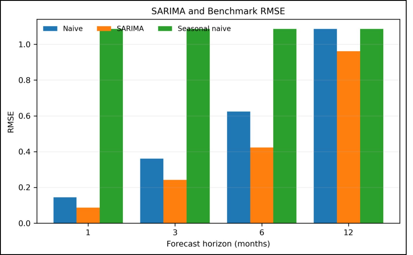
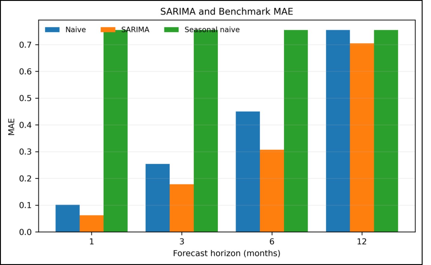
The naive benchmark results in significantly lower RMSE and MAE for periods of 1–6 months, which indicates high short-term persistence. Both benchmarks meet after 12 months as target aligned forecasts over the seasonal time horizon are the same as naive ones (Figs. 6 and 7).
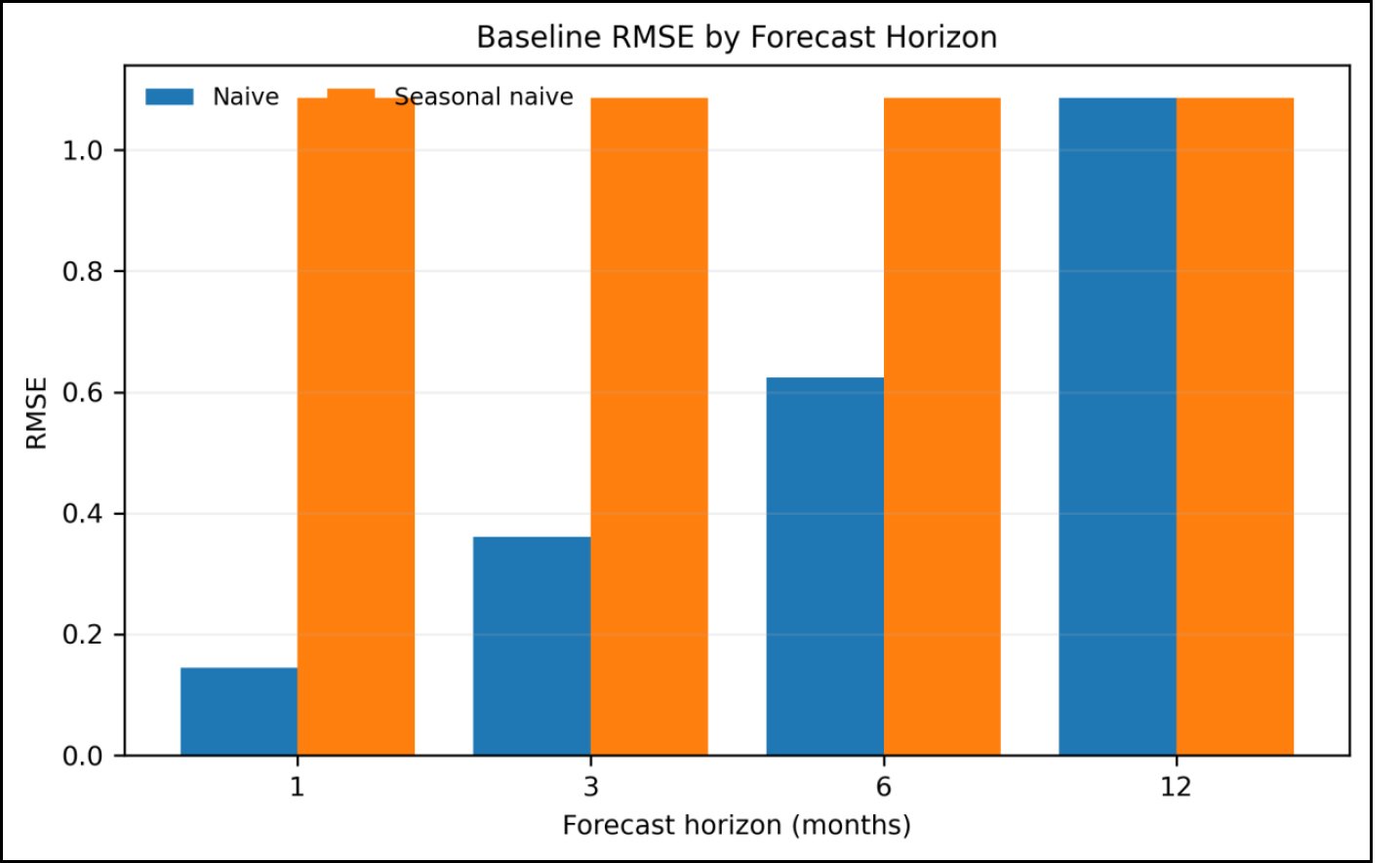
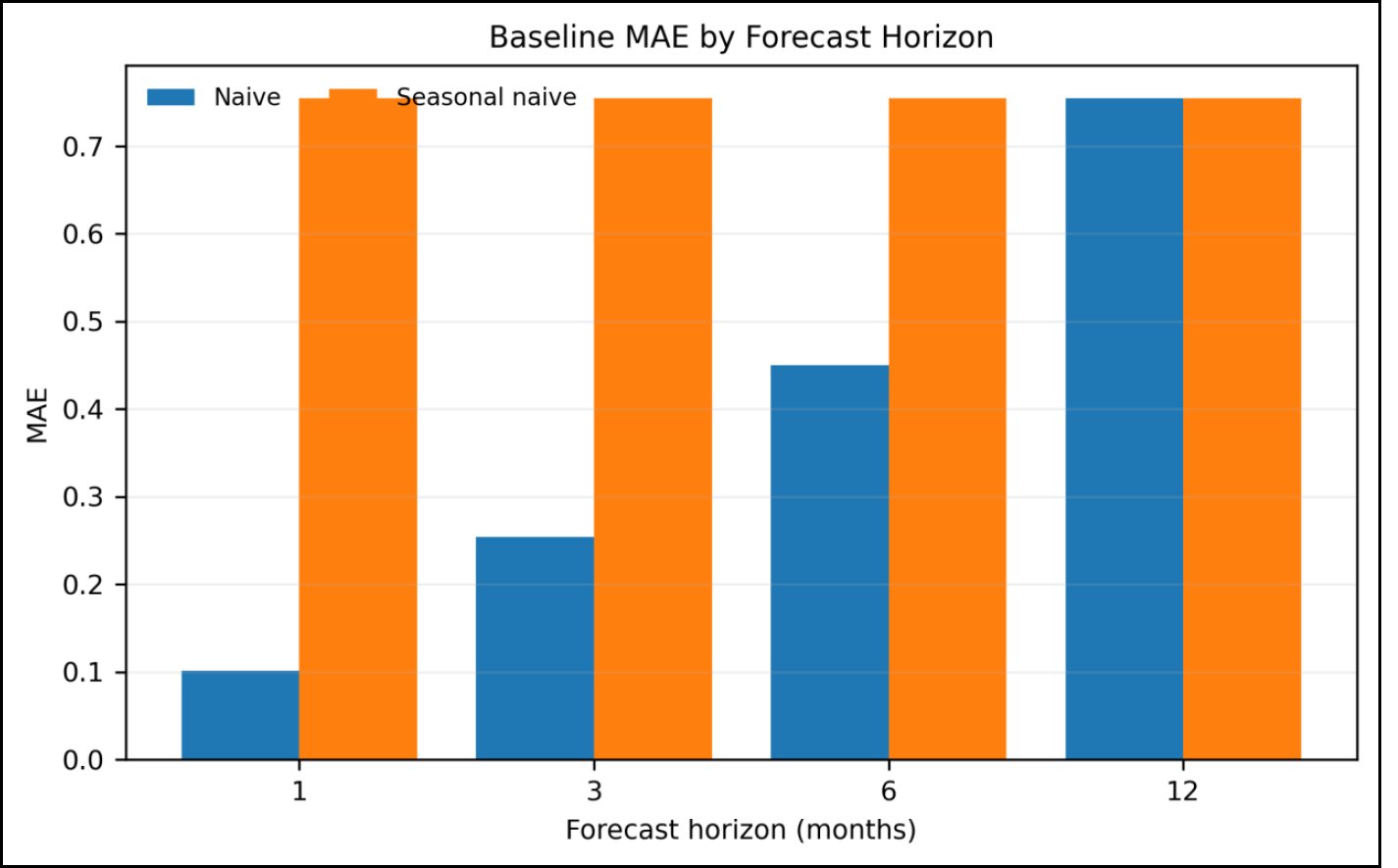
Fig. (6). RMSE of naive and seasonal-naive forecasts by horizon.

Fig. (7). MAE of naive and seasonal-naive forecasts by horizon.

4. RESULTS

4.1. Descriptive Patterns

CPI stickiness was high and erratic in the 1970s and early 1980s, fell during other decades and rose after 2020. The seasonal component is less in size when compared with the trend and remainder. The ACF is a decreasing curve, while the PACF is a good first-lag curve alone, so there is no reason to believe that the order of the SARIMA model can be determined by visual inspection.

4.2. Point-Forecast Accuracy

The descriptive RMSE and MAE values are the lowest for SARIMA at all horizons. Its RMSE values are 0.0869, 0.2420, 0.4229 and 0.9611 at 1, 3, 6 and 12 months, compared with 0.1940, 0.4314, 0.7564 and 1.3040 for XGBoost. Relative to the naive model, SARIMA reduces RMSE by 39.92%, 32.86%, 32.28% and 11.47%, respectively. In the reproduced analysis, XGBoost has higher RMSE than the naive benchmark at all four horizons. Table 9 shows that at 12 months the RMSE of naive and seasonal naive forecasts are the same by construction. In Section 4.3, the lower SARIMA loss when compared to the XGBoost loss comes from formal inference, at the 1-, 3-, and 6-month horizons, but is merely descriptive at the 12-month horizon because its corresponding DM-HLN test is not significant at the 5% level. This short-term bias is consequently stronger than difference of 12 months (Fig. 8).

Table 9. Forecast accuracy.

HorizonModelRMSEMAEMAPE (%)BiasError SD
1Naive0.14470.10134.240.00700.1449
1Seasonal naive1.08570.754632.190.10411.0834
1SARIMA0.08690.06242.82-0.01670.0855
1XGBoost0.19400.13607.44-0.03800.1908
3Naive0.36040.254110.620.02340.3605
3Seasonal naive1.08570.754632.190.10411.0834
3SARIMA0.24200.17818.25-0.07170.2317
3XGBoost0.43140.312715.96-0.08910.4231
6Naive0.62450.450518.790.05230.6239
6Seasonal naive1.08570.754632.190.10411.0834
6SARIMA0.42290.306914.07-0.07530.4172
6XGBoost0.75640.532327.04-0.13010.7470
12Naive1.08570.754632.190.10411.0834
12Seasonal naive1.08570.754632.190.10411.0834
12SARIMA0.96110.705234.57-0.21160.9399
12XGBoost1.30400.866442.80-0.33311.2639

Fig. (8). SARIMA and benchmark RMSE by forecast horizon.

Fig. (9) shows that SARIMA has lower MAE than the two benchmarks at each horizon in the descriptive results. The further away the time horizon, the more errors you will make in your forecast – the more significant the improvements over 1-6 month periods. The largest magnitude of error is the lower 12-month error, which is recorded by SARIMA, but this is described as a descriptive error ranking and not as inferential superiority.

Fig. (9). SARIMA and benchmark MAE by forecast horizon.

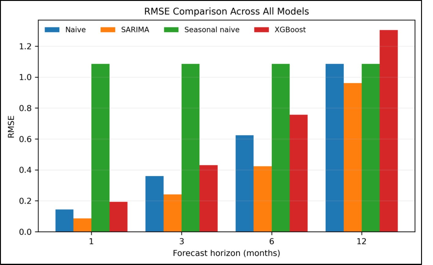
Fig. (10) validates the ranking in terms of RMSE at each horizon for all four models: SARIMA is the best model while the naive model is the worst model at each horizon. If the lower error of SARIMA is not a better model than its counterparts except the lower SARIMA, then the error value of it at 12-months can not be said to be statistically significant due to the comparison result of SARIMA vs. SARIMA-XGBoost DM-HLN has p = 0.0673. Here, the seasonal-naive benchmark does not fare well for shorter lead time, as is characteristic of this series (limited SVS).

Fig. (10). RMSE comparison across naive, seasonal-naive, SARIMA and XGBoost forecasts.

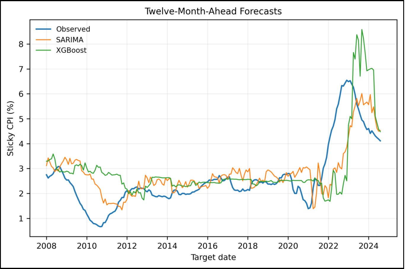
SARIMA provides a better fit to the observed path of Sticky CPI and has smoother forecasts over the assessment range. Both are weak during the post-2020 inflation spike. While XGBoost slightly underpredicts the growth rate in acceleration and then goes over the maximum, SARIMA has a more gradual adjustment, and stays fairly close to observed inflation (Fig. 11).

Fig. (11). Observed sticky CPI with 12-month SARIMA and direct XGBoost forecasts.

4.3. Formal Predictive-Accuracy Comparisons

SARIMA significantly outperforms XGBoost with respect to its squared-error loss, after adjustments for the 1 month, the 3 month, and the 6 month horizons over all 12 tests (p < 0.001, p = 0.0025 and p = 0.0241, respectively). On average, there is a smaller descriptive loss for SARIMA at 12 months, but this does not show up as a statistically significant difference (DM-HLN = -1.840, p = 0.0673). The previous finding of a statistically significant advantage for XGBoost over 12-months (Table 10) is not replicated. Raw p-value at 1 month is 0.0137, 3 months is 0.0108 and 6 months is 0.0102 but after an Holm all-test correction, the values for 1 month and 3 months remain significant, that for 6 months becomes 0.0625 and that for 12 months is not. After 1 month, XGBoost is much worse than naive, but after correcting all of the others are not significantly different from naive. This means that H1 is not supported as it does not have a model produced line with the lowest error.

Table 10. HLN-corrected diebold-mariano tests.

hComparisonMean loss diff.DM-HLNRaw pHolm: familyHolm: all 12Lower loss
1sarima vs xgboost-0.0301-5.9251.353e-085.412e-081.624e-07Sarima
1sarima vs naive-0.0134-4.5429.649e-063.859e-050.0001061Sarima
1xgboost vs naive0.01673.7460.0002350.000940.00235Naive
3sarima vs xgboost-0.1275-3.6980.0002810.00084290.002529Sarima
3sarima vs naive-0.0713-2.7360.0067840.020350.04749Sarima
3xgboost vs naive0.05621.7940.074280.22280.3363Naive
6sarima vs xgboost-0.3933-3.0040.0030090.0060170.02407Sarima
6sarima vs naive-0.2111-2.5860.010420.020840.06252Sarima
6xgboost vs naive0.18221.5190.13040.22280.3363Naive
12sarima vs xgboost-0.7767-1.8400.067270.067270.3363Sarima
12sarima vs naive-0.2550-1.1080.26920.26920.3363Sarima
12xgboost vs naive0.52171.6970.091280.22280.3363Naive

4.4. Predefined Pre-2020 and Post-2020 Periods

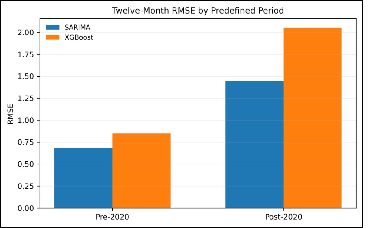
The errors observed in the 12 month period after January 2020 are significantly higher in all the models. Pre-2020, the naive model has the lowest descriptive RMSE (0.6117), followed by SARIMA (0.6846) and XGBoost (0.8486). The 95% moving-block bootstrap intervals for the difference between the SARIMA-XGBoost pre-2020 and the base period include 0: (-0.3902, 0.0887). Post-2020, SARIMA records RMSE 1.4471, compared with 2.0546 for XGBoost and 1.8021 for naive. SARIMA-XGBoost RMSE difference is -0.6075 and the 95% bootstrap interval is (-1.0879, -0.0943) indicating that the difference is not zero, thereby providing support for lower RMSE values for SARIMA in the prediction period after 2020 (Tables 11 and 12). It is a fixed time comparison that is not a structural break endogenously detected.

Table 11. Twelve-month accuracy by predefined target period.

PeriodModelnRMSEMAEMAPE (%)Bias
Pre-2020Naive1440.61170.471630.16-0.0195
Pre-2020Sarima1440.68460.510634.79-0.4201
Pre-2020Xgboost1440.84860.572444.54-0.4977
Post-2020Naive561.80211.482337.400.4218
Post-2020Sarima561.44711.205434.000.3246
Post-2020Xgboost562.05461.622538.320.0900

Table 12. Moving-block bootstrap RMSE intervals.

PeriodQuantityEstimate95% lower95% upper
Post-2020sarima rmse1.44711.02642.0849
Post-2020xgboost rmse2.05461.33802.8425
Post-2020rmse difference sarima minus xgboost-0.6075-1.0879-0.0943
Pre-2020sarima rmse0.68460.42120.9705
Pre-2020xgboost rmse0.84860.41511.2422
Pre-2020rmse difference sarima minus xgboost-0.1640-0.39020.0887

Unlike SARIMA, descriptively, before 2020 the RMSE of XGBoost is within the range of RMSEs drawn from boostrap interval when estimating the difference of their RMSEs. Both models suffer from much larger errors after 2020; the paired bootstrap interval over the difference excludes zero and SARIMA has the lower RMSE. In Fig. (12), therefore, the difficulty in forecasting is shown for particular periods but does not suggest the existence of a breakpoint in January 2020.

Fig. (12). Twelve-month SARIMA and XGBoost RMSE in the predefined pre-2020 and post-2020 periods.

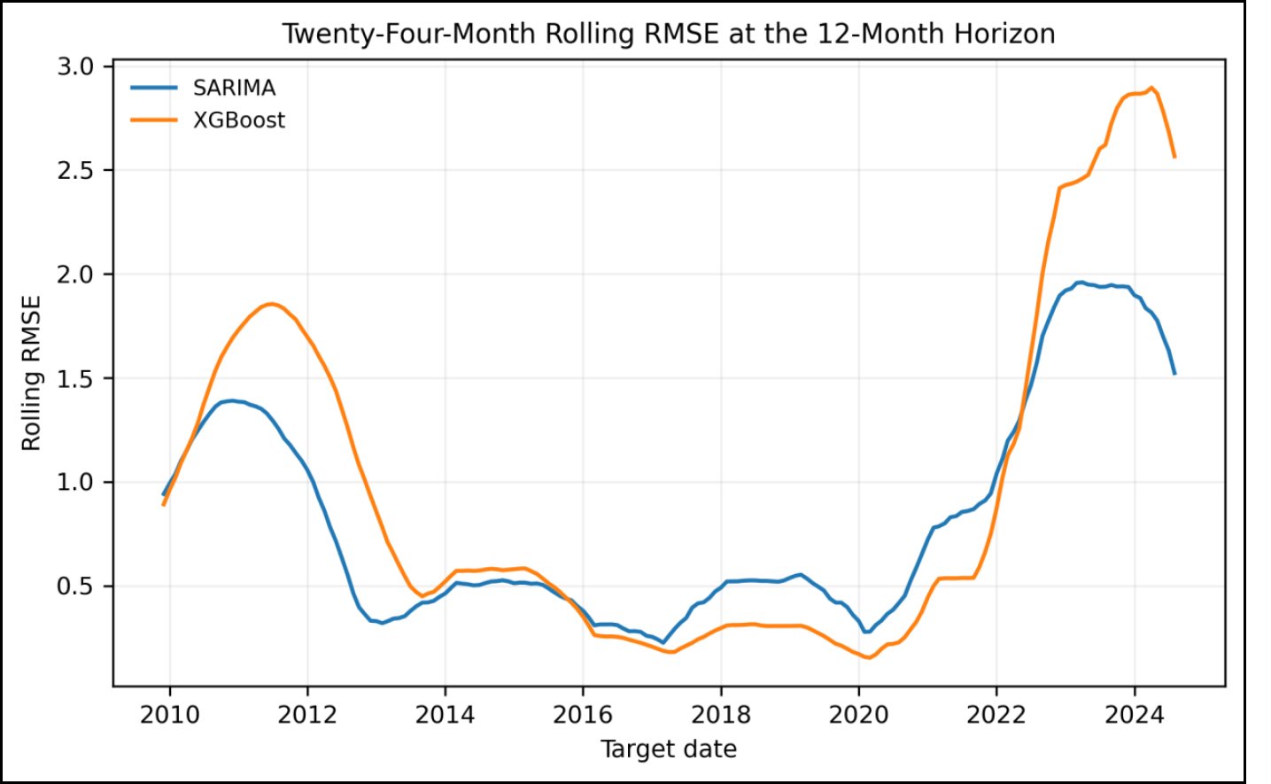
The 24-month rolling comparison shows that 12-month forecast errors rise sharply during the post-2020 episode for both methods. SARIMA’s rolling RMSE is lower than XGBoost’s over much of the displayed evaluation period, but the figure is descriptive and should not be interpreted as a formal test of a structural change or of time-varying statistical significance (Fig. 13).

Fig. (13). Twenty-four-month rolling RMSE for 12-month SARIMA and XGBoost forecasts.

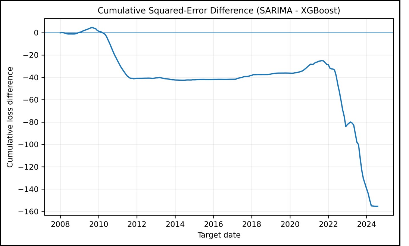
The cumulative squared-error difference is predominantly negative and declines sharply after 2022. Because the plotted quantity is SARIMA loss minus XGBoost loss, negative values indicate lower cumulative squared-error loss for SARIMA. The recent decline therefore shows that the cumulative descriptive loss gap moved further in SARIMA’s favour during the later inflation and disinflation episode (Fig. 14).

Fig. (14). Cumulative squared-error difference between SARIMA and XGBoost at the 12-month horizon. Positive values favour XGBoost; negative values favour SARIMA.

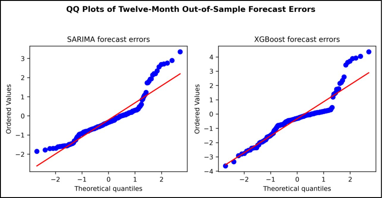
The distributions of forecast errors in- and out-of-sample are non-normal (heavy-tail behaviour) as evidenced by both QQ plots, especially in the tails. XGBoost has bigger extreme deviation in both extremes compared with SARIMA. The diagnostics suggest increased miss risk of large inflation movements and the need to use caution when using normality-based approximation to forecast-error inference (Fig. 15).

Fig. (15). Quantile-quantile plots of 12-month out-of-sample forecast errors.

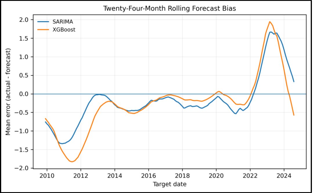
Rolling bias is highly time varying. In some previous periods of the evaluation, both models overpredict, but they approach zero around 2020, and then underpredict in the inflation acceleration period 2022-2023. XGBoost attains the higher positive-bias peak and SARIMA settles in slowly. Future predictions of the variables by XGBoost are increasingly biased towards overprediction, while SARIMA is slightly underpredictive by 2024 (Fig. 16).

Fig. (16). Twenty-four-month rolling bias of 12-month SARIMA and XGBoost forecasts.

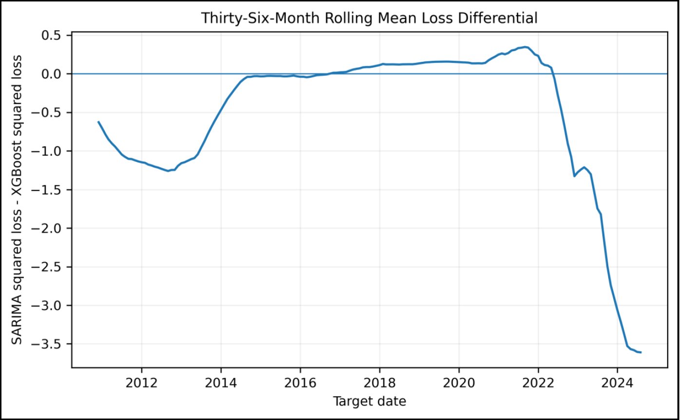
The rolling squared-loss difference is typically negative, suggesting that the squared-error loss of SARIMA is lower for much of the length of the window shown. There is a small positive interval between 2017 and 2022, suggesting that XGBoost shows a temporary descriptive improvement, but then the difference moves to a high negative interval. The relative change in loss over time is therefore useful to find in Fig. (17), but should not be used to replace the horizon specific DM-HLN inference presented in Table 10.

Fig. (17). Thirty-six-month rolling mean squared-loss differential. Negative values favour SARIMA.

4.5. Prediction-Interval Performance

Both interval systems are conservative systems. SARIMA 80% coverage ranges from 95.0% to 97.5%, and its 95% coverage ranges from 99.0% to 100.0%. The coverage of XGBoost is 80% at 88.0% to 96.5%, while all 95% empirical intervals cover 100% of targets. The high coverage is partly obtained by not calibrating the nominal values exactly (Table 13) but by using intervals. For XGBoost, these results are only for validation-calibrated empirical intervals, and should not be interpreted as finite-sample conformal guarantees.

Table 13. Prediction-interval coverage, width and score.

hModelNominalCoverageMean WidthMean Interval Score
1Sarima80%97.5%0.44350.4687
1Sarima95%99.0%0.67830.7011
1Xgboost80%90.0%0.69040.8185
1Xgboost95%100.0%1.70721.7072
3Sarima80%95.5%1.13361.2053
3Sarima95%99.0%1.73371.7677
3Xgboost80%88.0%1.43491.7217
3Xgboost95%100.0%3.64843.6484
6Sarima80%95.0%2.10362.1795
6Sarima95%100.0%3.21713.2171
6Xgboost80%91.0%3.02183.2738
6Xgboost95%100.0%6.21006.2100
12Sarima80%95.0%4.25514.5439
12Sarima95%99.5%6.50766.5644
12Xgboost80%96.5%6.95687.0975
12Xgboost95%100.0%12.051212.0512

This assessment shows that the SARIMA intervals are always more precise. At 12 months, its mean width is 80% and the interval mean scores are 4.2551 and 4.5439 respectively for XGBoost and its model. At the 95% level, mean widths are 6.5076 and 12.0512, respectively. The validation-calibrated empirical XGBoost intervals are especially conservative at long horizons due to the heterogeneous time periods in which the data has been validated and limited number of calibration errors.

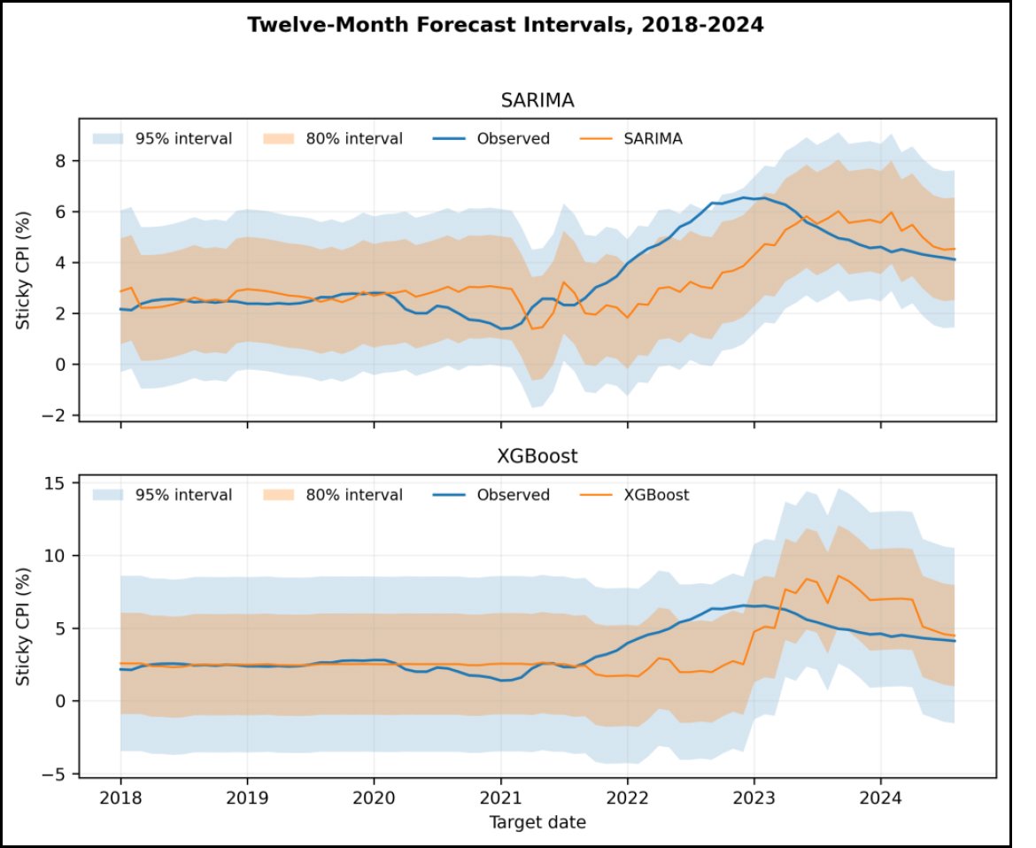
The 12-months time periods include most of the observed targets, but are conservative. The width of the bands of SARIMA is smaller in the period plotted and the path of inflation within the bands is closer. The validation-calibrated empirical intervals of XGBoost are wider, especially after 2022, which means that the sharpness of XGBoost is lower at the long horizon; XGBoost would not be using formal finite-sample conformal intervals (Fig. 18).

Fig. (18). Observed sticky CPI with 80% and 95% 12-month prediction intervals, 2018-2024.

4.6. Feature-Group Ablation and Importance

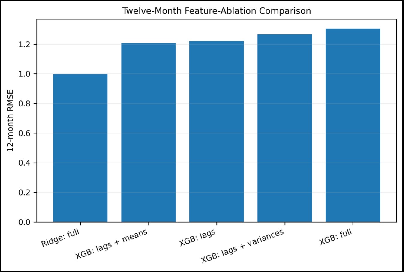
The three months of ablation results do not justify any benefits on nonlinear feature interaction or rolling variance for 12 months. The best RMSE value is for the full XGBoost model (1.3040). The RMSE is reduced slightly by adding rolling to lags (1.2205 to 1.2068) but increased by adding rolling variances to lags (1.2663). The descriptive results show that the achieved performance of the full feature-set of the ridge regression is the smallest of 0.9980 that surpassed the performance of all the XGBoost variants as well as the SARIMA method with 0.9611 (Table 14). Within the full XGBoost fit, lag 2, lag 1 and the three-month rolling mean have the largest gain-based importances. These importances are predictive diagnostics, not causal effects. The stronger ridge result suggests that the feature set contains useful predictive information, but nonlinear tree partitioning does not exploit it effectively in this sample.

Table 14. Twelve-month feature-ablation results.

SpecificationRMSEMAEMAPE (%)Bias
Ridge: full features0.99800.741635.55-0.2565
XGBoost: lags + means1.20680.810640.62-0.2878
XGBoost: lags only1.22050.813640.90-0.3106
XGBoost: lags + variances1.26630.845142.33-0.3521
XGBoost: full features1.30400.866442.80-0.3331

Fig. (19) shows that ridge regression with the full feature set has the lowest 12-month RMSE among the ablation specifications. Among the XGBoost variants, lags plus rolling means gives the lowest RMSE (1.2068), followed by lags only (1.2205), lags plus variances (1.2663) and the full specification (1.3040). These are descriptive accuracy differences; no separate inferential test establishes significant differences among the ablation variants.

Fig. (19). Twelve-month RMSE of XGBoost feature-group ablations and the ridge benchmark.

4.7. Forecast Combinations

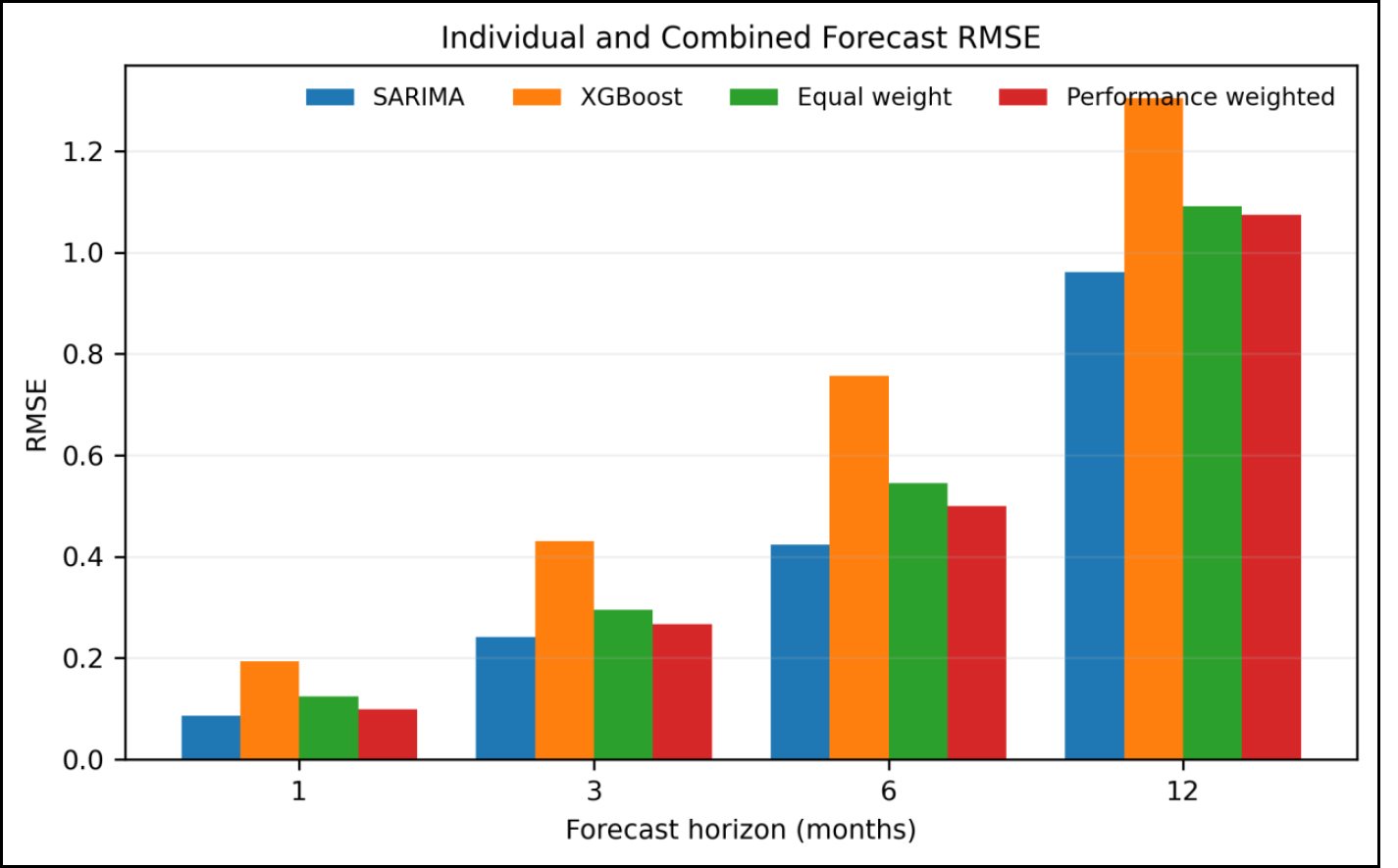
Both the equal-weight and rolling performance-weighted combinations have lower error than XGBoost, but neither has lower RMSE than SARIMA at any horizon. At 12 months, for example, equal-weight and performance-weighted RMSE values are 1.0915 and 1.0741, respectively, compared with 0.9611 for SARIMA. Forecast combinations may still be useful for robustness and disagreement monitoring, but their value should be established out of sample rather than assumed (Table 15).

Table 15. Individual and combined forecast accuracy.

hMethodRMSEMAEMAPE (%)
1Sarima0.08690.06242.82
1Xgboost0.19400.13607.44
1Equal Weight0.12480.08974.70
1Performance Weighted0.09970.07323.51
3Sarima0.24200.17818.25
3Xgboost0.43140.312715.96
3Equal Weight0.29550.214910.81
3Performance Weighted0.26680.19689.57
6Sarima0.42290.306914.07
6Xgboost0.75640.532327.04
6Equal Weight0.54470.379618.81
6Performance Weighted0.50030.348716.94
12Sarima0.96110.705234.57
12Xgboost1.30400.866442.80
12Equal Weight1.09150.763037.83
12Performance Weighted1.07410.753037.44

The lowest RMSE is recorded for SARIMA for all the horizons (Fig. 20). The performance-weighted combination of the forecasts has a much smaller descriptive RMSE than the equal-weight combination of the forecasts, as well as much smaller descriptive RMSE than XGBoost, in both cases. These do not outperform SARIMA, however, suggesting that it is not possible to get an error reduction by introducing the weaker XGBoost forecasting error.

Fig. (20). RMSE of individual and combined forecasts by horizon.

5. DISCUSSION

This study offers a more controlled and reproducible comparison of SARIMA with XGBoost for forecasting the Sticky Price Consumer Price Index Less Food and Energy (CPI-LFE) for the United States. Having standardized target dates, by fitting models into the analysis and the testing, which were separated, eliminated the choice of pre-evaluation model and the inference of the forecast accuracy, SARIMA is the model with the lowest RMSE and MAE over the four forecast horizons. Its RMSE values are 0.0869, 0.2420, 0.4229 and 0.9611 at 1, 3, 6 and 12 months, compared with 0.1940, 0.4314, 0.7564 and 1.3040 for XGBoost. More importantly, these results are based on comparing a full forecasting system that forecasts the SARIMA specification recursively, to a set of direct models, with each model being trained separately at each time horizon using XGBoost. These are not meant to be thought of in terms of a pure algorithm-family comparison where the multi-step forecasting strategy is the same.

The strongest inferential evidence for SARIMA occurs at the shorter horizons. The corrected DM-HLN tests show significantly lower SARIMA squared-error loss than XGBoost at 1, 3 and 6 months after the all-test Holm adjustment. This pattern is consistent with the strong persistence of Sticky CPI and with prior evidence that parsimonious autoregressive models can be difficult to beat when recent inflation contains substantial predictive information [3, 31]. The ACF declines slowly and the PACF has a strong first-lag response, indicating that recent Sticky CPI is closely related to near-term values. SARIMA represents this dependence parsimoniously, whereas XGBoost must estimate multiple threshold-based relationships from a comparatively modest univariate macroeconomic sample.

The inferential evidence is less strong, but at 12 months, SARIMA also has the minimum point-forecast error. The two-tailed p-value of the SARIMA-XGBoost DM-HLN statistic is 0.0673 and the statistic is -1.840. Thus, the 12 month upward or downward deviation from the est line must be described as “descriptive” error of a lower or higher SARIMA, not as “statistical” 5% level error. The hypothesized horizon-specific ranking reversal is therefore not replicated: There is a prominent decrease in forecast accuracy at increased horizons, but descriptively lower error model does not switch.

As with the feature-ablation analysis, there is no evidence that nonlinear lag interactions or rolling variances offer better medium-term forecasting abilities. The lags plus rolling combination improves the RMSE from 1.2205 at 12 months to 1.2068, while rolling variances brings RMSE up to 1.2663, and the full specification of SMOOTH_XGBOOST has the highest RMSE among the three options of 1.3040 at 12 months. Using the full feature set for the same ridge regression obtains RMSE value 0.9980 which is smaller than all the variants of XGBoost and is close to SARIMA’s RMSE 0.9611. In this example the feature set therefore provides useful information for prediction, but in this case this is better represented in the linear relations, regularised by L1, than in the nonlinear partitions of the trees.

The pre-2020/post-2020 comparison is pre-defined and shows that it is not the case that the latter inflation episode is more extreme than the pre-2020 one, but merely that it is more difficult to predict for all models. Naive model (before 2020) has the lowest RMSE for describing the time series, followed by SARIMA and XGBoost, and includes the zero in the bootstrap wide-confidence interval (WC-I) of the difference between the log RMSE of SARIMA and XGBoost. Post-2020, SARIMA records RMSE 1.4471 compared with 1.8021 for naive and 2.0546 for XGBoost. Paired moving-block bootstrap confidence interval is (-1.0879, -0.0943) and the difference is in favor of SARIMA and equals -0.6075. SARIMA and XGBoost both have a tendency to underpredict inflation after 2020, but also underpredict it from 2016 until the 2019 period, indicating that some amount of “lagged sticky CPI” is insufficient to successfully predict inflation gains.

The prediction-interval results reinforce the necessity of rather careful interpretation of the uncertainty associated with their predictions. For both systems, conservative intervals are found, and intervals based on SARIMA model are found to be narrower intervals with the lower mean interval score. The mean width at 12 months is 4.2551, and the mean interval score is 4.5439 for SARIMA and 6.9568, 7.0975 for XGBoost. In XGBoost, they are simply intervals that are informed by data for validation purposes, not formal finite-sample conformal intervals and are notably wider than usual with long time horizons. The coverage is thus to be understood in combination with width and interval score [23, 24].

Even though the error rate of the forecast combinations is smaller than that of XGBoost, there is no improvement in this sample. Similar equal-weight and rolling performance-weighted combinations achieve RMSE equal to 1.0915 and 1.0741 at 12 months respectively, and 0.9611 for SARIMA. Combination forecasts could still be valuable in the role of robustness checks and disagreement signals, but this should be done by using only prior out-of-sample information to evaluate the weights and forecast performance of the components [25].

In a “forecasting-practice” perspective, the results do not favour an automatic model switching based on the horizon. SARIMA is the best in-sample univariate point-forecast model; the other models could be kept as a complementary diagnosis. However, when there are significant discrepancies between the models, it could be an indicator of varying data conditions and can encourage scenario analysis instead of automatic changes of models [26, 27]. To monitor the average point error, a rolling bias, width of the intervals, interval score, and interval score dispersion should also be used.

LIMITATIONS

The study is univariate, and the data that is being analysed is current vintage FRED data, not archived real-time vintages, thus the exercise is pseudo-out-of-sample not real out-of-sample. Second, SARIMA is recursive, while XGBoost is direct: The comparison is therefore for whole forecasting systems rather than algorithm family alone. Third, the lowest AIC SARIMA model still has statistically significant residual autocorrelation. This does not invalidate the out-of-sample ranking evidence as before because the comparative inference is based on common-target forecast errors with HAC adjusted, but it shows that the model is imperfectly adequate and should not be taken as a reason to be cautious when interpreting the intervals of SARIMA’s model. Fourth, the January 2020 split is predefined and is not an estimated breakpoint. Fifth, XGBoost intervals are validation-calibrated empirical intervals and remain conservative. Finally, the findings concern one U.S. inflation series and should not be generalised to multivariate macroeconomic forecasting settings, where XGBoost may have access to substantially richer predictive information and model rankings may differ. Future research should focus on real-time vintages, extended macroeconomic predictions, alternative measures of inflation, more comprehensive statistical specifications, and formally estimated periods and adapted probability forecasting techniques.

CONCLUSION

This study provides a leakage-controlled, multi-horizon comparison of SARIMA and XGBoost for forecasting the U.S. Sticky Price Consumer Price Index Less Food and Energy. The present-to-vintage data has 680 observations that are monthly data, from January 1968 until August 2024. The model development is limited to January 1968-December 2007 and the pseudo out-of-sample evaluation takes place at the same 200 target months for each horizon from January 2008 – August 2024, with only model tuning using SARIMA order being performed between these months. Only the model development covers the months of January 1968-December 2007, and only the tuning of XGBoost results applies to the same 200 target months at each horizon, 1-24, from January 2008 till August 2024.

Reproducing results do not agree with the initial proposed 12-month XGBoost benefit. The RMSE and MAE values of SARIMA are minimum over 1, 3, 6 and 12 months. At 1, 3 and 6 months after the Holm-adjustment all-test corrected DM-HLN, SARIMA performs better than XGBoost. For descriptive error, SARIMA has lower error, however the difference is not statistically significant at 5% (DM-HLN -1.840, p = 0.0673). It is therefore not confirmed that the hypothesised horizon-specific ranking reversal is true.

The ‘post 2020’ analysis displayed above is a pre-defined by the models, and becomes more challenging in the final inflation episode. Both SARIMA and XGBoost have smaller 12-month RMSE during this time, and there is no evidence of a formally detected structural break in this period in the paired moving-block bootstrap interval for the RMSE difference. When it comes to nonlinear lag interaction and rolling variance, feature ablation does not show any benefit from those features when directly tested against the complete set of predictors and, remarkably, the best-performing model is still a ridge regression using the same set of basis features as XGBoost.

SARIMA also yields tighter model-based prediction intervals that have lower interval scores, and XGBoost’s wider intervals are conformal intervals with some form of empirical calibration as opposed to intervals that are finite sample guarantees. The combinations of forecasts further reduce the error of XGBoost, but not beyond the error of SARIMA. Note that SARIMA provides the best univariate benchmark for Sticky CPI in this assessment, and naive and combined forecasts are still useful in addition to the model-disagreement diagnostics for model robustness. Results cannot be extrapolated to the context of data-rich multivariate macroeconomic forecasting where machine learning models may make use of far more predictive information. Other factors such as real-time vintages, broader sets of macroeconomic variables, alternate measures of inflation, formally estimated break dates, and adaptive, probabilistic forecasting techniques should be measured in the future.

LIST OF ABBREVIATIONS

CPI-LFE

=

Consumer Price Index Less Food and Energy

XGBoost

=

Extreme Gradient Boosting

SARIMA

=

Seasonal Autoregressive Integrated Moving Average

Sticky CPI

=

Sticky Price Consumer Price Index

AUTHOR’S CONTRIBUTION

S.S. contributed to the study conceptualization and design, model implementation, experimental evaluation, data analysis, methodology, manuscript drafting, and critical revision.

ETHICAL APPROVAL & INFORMED CONSENT

Ethical approval was not required for this study because it used publicly available historical macroeconomic data and did not involve human participants, personal data, or primary data collection. Therefore, informed consent was not applicable.

AVAILABILITY OF DATA AND MATERIALS

This data source is publicly accessible from a FRED resource: CORESTICKM159SFRBATL [26]. Analysis is done in Python, Pandas, Numpy, Statsmodels, Scikit learn, XGboost, SciPy and Matplotlib. A fixed random seed of 42 is used for stochastic procedures. The figure package consists of 20 300-dpi PNG sources and an inventory file that names the figure generation script.

FUNDING

None.

CONFLICT OF INTEREST

The author declares that there is no conflict of interest regarding the publication of this article.

ACKNOWLEDGEMENTS

Declared none.

DECLARATION OF AI

No Artificial Intelligence (AI) tools were used to collect, process, analyze, model, or interpret the data, or to generate the results presented in this manuscript. The forecasting models, statistical analyses, and interpretation of findings were conducted by the author using the specified methodological procedures.

REFERENCES

[1] Iftikhar, F. Khan, P. C. Rodrigues, A. A. Alharbi, and J. Allohibi, “Forecasting of inflation based on univariate and multivariate time series models: An empirical application,” Mathematics, vol. 13, no. 7, Art. no. 1121, 2025,
https://doi.org/10.3390/math13071121

[2] Kiley and F. S. Mishkin, “Central banking post crises,” NBER Working Paper No. 32237, 2024,
https://doi.org/10.3386/w32237

[3] H. Stock and M. W. Watson, “Why has US inflation become harder to forecast?” J. Money, Credit Bank., vol. 39, no. s1, pp. 3-33, 2007,
https://doi.org/10.1111/j.1538-4616.2007.00014.x

[4] J. Blanchard and B. S. Bernanke, “What caused the US pandemic-era inflation?” NBER Working Paper No. 31417, 2023,
https://doi.org/10.3386/w31417

[5] Ball, D. Leigh, and P. Mishra, “Understanding US inflation during the COVID-19 era,” MF Working Papers 2022, 2022,
https://doi.org/10.5089/9798400225390.001

[6] F. Bryan and B. Meyer, “Are some prices in the CPI more forward looking than others? We think so,” Econ. Comment., no. 2010-02, 2010,
https://doi.org/10.26509/frbc-ec-201002

[7] J. Tashman, “Out-of-sample tests of forecasting accuracy: An analysis and review,” Int. J. Forecast., vol. 16, no. 4, pp. 437-450, 2000,
https://doi.org/10.1016/S0169-2070(00)00065-0

[8] J. Hyndman and G. Athanasopoulos, Forecasting: Principles and Practice, 2nd ed. Melbourne, Australia: OTexts, 2018, Available from: https://otexts.com/fpp2/

[9] Bergmeir, R. J. Hyndman, and B. Koo, “A note on the validity of cross-validation for evaluating autoregressive time series prediction,” Comput. Stat. Data Anal., vol. 120, pp. 70-83, 2018,
https://doi.org/10.1016/j.csda.2017.11.003

[10] Koutsandreas, E. Spiliotis, F. Petropoulos, and V. Assimakopoulos, “On the selection of forecasting accuracy measures,” J. Oper. Res. Soc., vol. 73, no. 5, pp. 937-954, 2022,
https://doi.org/10.1080/01605682.2021.1892464

[11] E. P. Box, G. M. Jenkins, G. C. Reinsel, and G. M. Ljung, “Time Series Analysis: Forecasting and Control”. John Wiley & Sons, 2015, Available from: https://www.wiley.com/en-us/shop/general-introductory-statistics/time-series-analysis-forecasting-and-control-5th-edition-p-9781118675021

[12] J. Hyndman and Y. Khandakar, “Automatic time series forecasting: The forecast package for R,” J. Stat. Softw., vol. 27, no. 3, pp. 1-22, 2008,
https://doi.org/10.18637/jss.v027.i03

[13] A. Dickey and W. A. Fuller, “Distribution of the estimators for autoregressive time series with a unit root,” J. Amer. Stat. Assoc., vol. 74, no. 366a, pp. 427-431, 1979,
https://doi.org/10.1080/01621459.1979.10482531

[14] Kwiatkowski, P. C. B. Phillips, P. Schmidt, Y. Shin, “Testing the null hypothesis of stationarity against the alternative of a unit root: How sure are we that economic time series have a unit root? ,” J. Econometrics, vol. 54, no. 1-3, pp. 159-178, 1992,
https://doi.org/10.1016/0304-4076(92)90104-Y

[15] Fouladvand, M. Noshad, M. K. Goldstein, V. J. Periyakoil, and J. H. Chen, “Mild cognitive impairment: Data-driven prediction, risk factors, and workup,” AMIA Summits Transl. Sci. Proc., vol. 2023, p. 167, 2023, Available from: https://pubmed.ncbi.nlm.nih.gov/37350911

[16] C. Medeiros, G. F. Vasconcelos, Á. Veiga, and E. Zilberman, “Forecasting inflation in a data-rich environment: The benefits of machine learning methods,” J. Bus. Econ. Stat., vol. 39, no. 1, pp. 98-119, 2021,
https://doi.org/10.1080/07350015.2019.1637745

[17] G. Coulombe, M. Leroux, D. Stevanovic, and S. Surprenant, “How is machine learning useful for macroeconomic forecasting?” J. Appl. Econometrics, vol. 37, no. 5, pp. 920-964, 2022,
https://doi.org/10.1002/jae.2910

[18] Bell, I. Solano-Kamaiko, O. Nov, and J. Stoyanovich, “It’s just not that simple: An empirical study of the accuracy-explainability trade-off in machine learning for public policy,” in Proc. 2022 ACM Conf. Fairness, Accountability, Transparency, 2022, pp. 248-266,
https://doi.org/10.1145/3531146.3533090

[19] Perez-Bernabeu and O. Polat, “AI and machine learning in macroeconomic forecasting: A systematic review of models, trends, and challenges,” in Proc. 2025 IEEE Int. Conf. Eng., Technol. Innov. (ICE/ITMC), 2025, pp. 1-9,
https://doi.org/10.1109/ICE/ITMC65658.2025.11106520

[20] X. Diebold and R. S. Mariano, “Comparing predictive accuracy,” J. Bus. Econ. Stat., vol. 20, no. 1, pp. 134-144, 2002,
https://doi.org/10.1198/073500102753410444

[21] Harvey, S. Leybourne, and P. Newbold, “Testing the equality of prediction mean squared errors,” Int. J. Forecast., vol. 13, no. 2, pp. 281-291, 1997,
https://doi.org/10.1016/S0169-2070(96)00719-4

[22] K. Newey and K. D. West, “A simple, positive semi-definite, heteroskedasticity and autocorrelation consistent covariance matrix,” Appl. Econometrics, vol. 55, no. 3, pp. 703-708, 1987,
https://doi.org/10.2307/1913610

[23] Gneiting and A. E. Raftery, “Strictly proper scoring rules, prediction, and estimation,” J. Amer. Stat. Assoc., vol. 102, no. 477, pp. 359-378, 2007,
https://doi.org/10.1198/016214506000001437

[24] Xu and Y. Xie, “Conformal prediction interval for dynamic time-series,” in Proc. Int. Conf. Mach. Learn., 2021, pp. 11559-11569, Available from: https://proceedings.mlr.press/v139/xu21h.html

[25] Wang, R. J. Hyndman, F. Li, and Y. Kang, “Forecast combinations: An over 50-year review,” Int. J. Forecast., vol. 39, no. 4, pp. 1518-1547, 2023,
https://doi.org/10.1016/j.ijforecast.2022.11.005

[26] Federal Reserve Bank of Atlanta, “Sticky Price Consumer Price Index Less Food and Energy [CORESTICKM159SFRBATL],” FRED, Federal Reserve Bank of St. Louis, 2026, Available from: https://fred.stlouisfed.org/series/CORESTICKM159SFRBATL

[27] M. Maiga, “Empirical approach to modelling and forecasting inflation using ARIMA model: Evidence from Tanzania,” J. Agric. Stud., vol. 12, no. 2, pp. 58-76, 2024,
https://doi.org/10.5296/jas.v12i2.21695

[28] He, M. U. Rahman, and C. Xie, “Information overflow between monetary policy transparency and inflation expectations using multivariate stochastic volatility models,” Appl. Math. Sci. Eng., vol. 31, no. 1, Art. no. 2253968, 2023,
https://doi.org/10.1080/27690911.2023.2253968

[29] L. Bihan, D. Leiva-León, and M. Pacce, “Underlying inflation and asymmetric risks,” Rev. Econ. Stat., pp. 1-45, 2024,
https://doi.org/10.1162/rest_a_01522

[30] Koziol, “Mapping monetary transmission: Housing, CPI measurement and the two faces of inflation,” SSRN, 2026,
https://doi.org/10.2139/ssrn.7040338

[31] Faust and J. H. Wright, “Forecasting inflation,” in Handbook of Economic Forecasting, vol. 2, G. Elliott and A. Timmermann, Eds. Amsterdam, The Netherlands: Elsevier, 2013, pp. 2-56,
https://doi.org/10.1016/B978-0-444-53683-9.00001-3

[32] Alomani, M. Kayid, and M. F. Abd El-Aal, “Global inflation forecasting and uncertainty assessment: Comparing ARIMA with advanced machine learning,” J. Radiat. Res. Appl. Sci., vol. 18, no. 2, Art. no. 101402, 2025,
https://doi.org/10.1016/j.jrras.2025.101402

Insert math as
Block
Inline
Additional settings
Formula color
Text color
#333333
Type math using LaTeX
Preview
\({}\)
Nothing to preview
Insert