

pdpublishers.com

Article ID: PD2601208004

Views: 421
Volume 1 (2026)
Published 25 Jul 2026

A Comparative Evaluation of Statistical, Hybrid, and Deep Learning Models for Short-Term Electricity Demand Forecasting in The United Kingdom

📚 Cited by: 0

⬇ Downloads: 12


Authors

1Department of Statistics, King Abdulaziz University, Jeddah, Saudi Arabia

Article History:

Received: 19 May, 2026

Accepted: 09 July, 2026

Revised: 19 June, 2026

Published: 25 July, 2026

ABSTRACT:

Introduction: Accurate short-term electricity demand forecasting is essential for power-system reliability, generation scheduling, reserve planning, and renewable-energy integration. This study presents a controlled comparative evaluation of statistical, recurrent deep learning, convolutional-recurrent, and residual hybrid models for short-term electricity-demand forecasting in the United Kingdom using a publicly available UK/England-Wales electricity-demand dataset covering 2009–2022. The evaluated models include Naïve Persistence, Seasonal Naïve, Holt-Winters, ARIMA, SARIMA, Long Short-Term Memory, Gated Recurrent Unit, CNN-LSTM, and Hybrid ARIMA-LSTM.

Methodology: A chronological validation strategy was adopted to prevent temporal leakage, with 2009–2019 used for training, 2020–2021 for validation, and 2022 for out-of-sample testing. Model performance was assessed using RMSE, MAE, MAPE, and sMAPE on a consistent normalised test-set scale only as secondary operational interpretations where explicitly stated.

Results: The diagnostic baseline results showed that Naïve Persistence achieved low numerical error because it simply carried forward the most recent observation; however, it was retained only as a persistence benchmark and was not ranked as a trainable forecasting architecture. Among the implemented trainable models, GRU achieved the strongest performance among the implemented trainable forecasting architectures with RMSE = 0.027, MAE = 0.021, MAPE = 0.053, and sMAPE = 5.23%, followed closely by LSTM. CNN-LSTM remained competitive but did not outperform the pure recurrent models. Hybrid ARIMA-LSTM improved over ARIMA and SARIMA, achieving RMSE = 0.046, MAE = 0.038, MAPE = 0.099, and sMAPE = 9.54%, but it did not outperform GRU or LSTM.

Conclusion: These findings show that residual hybridisation can improve classical statistical baselines, but it should not be assumed to be superior to well-tuned recurrent neural networks. The main contribution of this study is a reproducible UK-focused benchmarking framework that clarifies model-selection trade-offs for electricity-demand forecasting and smart-grid analytics.

Keywords: Electricity load forecasting; time-series forecasting; short-term electricity demand; arima-lstm hybrid; gated recurrent unit; deep learning; renewable energy integration; smart grid analytics.

1. INTRODUCTION

Energy demand forecasting is an important factor to attain reliability, stability and efficiency of the existing power systems. Real-time balancing of supply and demand is supported by accurate forecasting and this assists grid operators to avoid shortages, overproduction and reduce operation costs [1]. In addition, an accurate forecast supports the long-term planning of energy, investing in infrastructure, and optimizing distributed energy resources [2]. It is also obligatory in the integration of renewable sources of energy including wind and solar that also have the issue of intermittency that affect stability of the grid. With the help of predicting patterns of consumption, utilities can be in a better position to manage variability in renewable resources, decrease reliance on fossil-based fuels, and attain a higher level of sustainability [3].

This paper offers an innovative idea as it utilises a nation-wide UK electricity demand dataset (2009-2022) with a hybrid deep learning algorithm, ARIMA-LSTM, to boost short term demand predictions. This approach uses linear and non-linear dependencies, which is very important in improving the accuracy of the forecasts because grid stability and the successful integration of renewable energy depend on this criterion. The demand of electricity in the UK undergoes drastic seasonal and intertemporal variability with the highest demand during winter because of the need to heat places and low demand during summer because of low demand [4]. The weather and holidays are also extreme factors that interfere with consumption patterns which are hard to forecast. Also, the increasing ratio of the renewable energy as the UK transitions to the low-carbon energy system brings increased uncertainty to the generation and demand. The complex, nonlinear, and dynamic nature of energy consumption data relationships necessitates more advanced forecasting models [5].

Some of the UK research on electricity demand forecasting, including Athanasopoulou et al. [6], have concentrated on the short-term predictions of electricity demand with the hybrid model based on LSTM and feature engineering. Although these studies are more accurate, they are mainly focused on short-term forecasting (daily-weekly) and utilise only one-paradigm approach. Also, there are a lot of studies that employ incoherent validation and they fail to investigate short-term prediction which is essential in incorporating renewable energy and operating the grid. In contrast to those studies, this research is based on a long-horizon and multi-paradigm approach where classical (ARIMA, SARIMA) and deep learning models (LSTM, GRU, CNN-LSTM) are tested based on a reproducible validation procedure.

Auto-Regressive Integrated Moving Average (ARIMA) and Seasonal Auto-regressive integrated Moving Average (SARIMA). These are traditional models that have been extensively used in energy forecasting since they can be used to capture linear trends and seasonality. Nevertheless, these models assume stationarity, as well as linearity, which is why they are not as useful when it comes to non-linear and non-stationary contemporary energy demand data [7]. The algorithms also have limitations due to the manual parameter optimization requirement and cannot scale to dynamic forecasting problems.

One of the strategies used to deal with some of these problems has been the use of machine learning methods like the random forests and the support vectors machine to model the nonlinear relationships in data. Nevertheless, these models are often not designed to deal with sequential data, as they require the time-varying memory in order to predict the long-term forecast [8, 9]. Deep learning algorithms, specifically the Long Short-Term Memory (LSTM) networks have conversely performed very well compared to the old algorithms such as ARIMA and Prophet when used to perform the energy prediction task [10, 11]. In any case, LSTM models require huge amounts of data and may have interpretability and scalability issues when handling small datasets.

Although previous studies have examined electricity demand forecasting using statistical, machine learning, hybrid, and deep learning models, important gaps remain. Many studies evaluate a limited group of models rather than comparing statistical, hybrid, and recurrent deep learning approaches under the same forecasting protocol [2, 4]. Several UK-focused studies also use narrower validation windows, limited model families, or inconsistent splitting strategies, which makes it difficult to determine whether reported improvements are caused by model architecture or by evaluation design. In addition, hybrid ARIMA-LSTM models are often assumed to be superior because they combine linear and nonlinear modelling, but there is limited evidence showing whether this advantage remains when they are compared directly with GRU, LSTM, and CNN-LSTM under identical chronological validation conditions.

The objectives of this study are:

To develop statistical and persistence baselines, including Naïve Persistence, Seasonal Naïve, Holt-Winters, ARIMA, and SARIMA, for short-term electricity-demand forecasting.

To implement recurrent and convolutional-recurrent deep learning models, including LSTM, GRU, and CNN-LSTM, to capture nonlinear temporal dependencies in UK electricity demand.

To construct a residual Hybrid ARIMA-LSTM model that combines linear ARIMA forecasting with nonlinear LSTM-based residual correction.

To evaluate all implemented models using the same chronological train-validation-test split and the same normalised test-set evaluation scale, while interpreting diagnostic persistence baselines separately from trainable forecasting architectures.

To assess statistical differences in forecast accuracy using Diebold-Mariano tests and examine robustness across seasonal and operational subsets.

This study addresses the need for a controlled and reproducible comparison of short-term electricity-demand forecasting models for the UK/England-Wales electricity-demand setting. The novelty of the paper is not the introduction of a completely new forecasting architecture. Rather, the contribution lies in providing a fair empirical benchmark in which statistical, recurrent deep learning, convolutional-recurrent, and residual hybrid models are evaluated under the same chronological validation design. It compares Naïve Persistence, Seasonal Naïve, Holt-Winters, ARIMA, SARIMA, LSTM, GRU, CNN-LSTM, and Hybrid ARIMA-LSTM using the same pre-processing, validation, and evaluation pipeline. The novelty of the paper is not the proposal of a completely new forecasting architecture. Instead, the contribution lies in providing controlled empirical evidence on how statistical, hybrid, and deep learning models behave under the same UK electricity-demand forecasting setting. This is important because the results show that Hybrid ARIMA-LSTM improves over ARIMA and SARIMA but does not outperform the best recurrent model, GRU.

The contributions of this study are threefold. First, it provides a controlled UK-focused benchmarking framework comparing persistence baselines, classical statistical models, recurrent deep learning models, convolutional-recurrent models, and residual hybrid models using the same chronological train-validation-test protocol. Second, it evaluates whether residual ARIMA-LSTM hybridisation provides meaningful improvement over classical ARIMA and SARIMA models and whether this improvement remains competitive against well-tuned recurrent neural networks. Third, it reports model performance using a consistent normalised test-set scale and selected Diebold-Mariano forecast-comparison tests to support transparent model selection for electricity-demand forecasting and smart-grid analytics. Diagnostic persistence baselines are reported separately because they do not learn trainable temporal, seasonal, or nonlinear demand relationships.

2. LITERATURE REVIEW

2.1. Machine Learning Models

With the introduction of Machine Learning (ML), the forecasting toolkit has been expanded with flexible and non-parametric algorithms that can be used to model nonlinear relationships that are hard to model [12, 13]. Random Forests (RF), Gradient Boosted Trees (GBT/XGBoost) and Support Vector Regression (SVR) methods have the ability to use large amounts of engineered features, such as historic consumption lags, temperature, humidity, calendar effects, and economic factors to further raise predictive power [14, 15].

Machine learning methods such as Random Forest, XGBoost, and Support Vector Regression have been widely used in energy-demand forecasting because they can model nonlinear relationships between lagged demand, calendar indicators, weather conditions, and other contextual variables [16]. These models are particularly useful when forecasting is treated as a tabular supervised-learning problem with carefully engineered lag, rolling, and calendar features [17, 18]. However, such models do not have an intrinsic sequential memory mechanism and therefore depend heavily on manual feature engineering to represent temporal dependence [19].

Transformer-based time-series models, including Temporal Fusion Transformer, Informer, and Autoformer, have also become important forecasting benchmarks because they are designed to model long-range temporal dependencies and multi-horizon structures [20]. These architectures are especially relevant for extended-horizon and probabilistic forecasting tasks. However, the present study focuses on classical statistical models, recurrent deep learning models, convolutional-recurrent models, and residual ARIMA-LSTM hybrid modelling because its central objective is to evaluate whether residual hybridisation improves forecasting performance relative to commonly used statistical and recurrent neural forecasting approaches under a controlled UK electricity-demand forecasting framework [21].  These models are discussed only to position the study within the broader forecasting literature and were not part of the empirical benchmark. Table 1.

Table 1. Implemented and non-implemented model scope.

Model GroupModels DiscussedImplemented in this Study?Reason
Persistence baselinesNaïve Persistence, Seasonal NaïveYesUsed as diagnostic lower-bound benchmarks for persistence and seasonality
Classical statistical modelsHolt-Winters, ARIMA, SARIMAYesRepresent interpretable linear, smoothing, and seasonal forecasting approaches
Recurrent deep learning modelsLSTM, GRUYesCapture nonlinear sequential dependencies in electricity-demand data
Convolutional-recurrent modelCNN-LSTMYesTests whether local temporal feature extraction improves recurrent forecasting
Residual hybrid modelHybrid ARIMA-LSTMYesEvaluates whether ARIMA-based linear forecasting plus LSTM residual correction improves accuracy
Tree-based machine learningRandom Forest, XGBoostNoDiscussed only as background; excluded to keep the empirical benchmark focused
Kernel-based machine learningSVRNoDiscussed only as background; not part of the implemented model family
Transformer-based forecastingTemporal Fusion Transformer, Informer, AutoformerNoRecognised as future benchmarks; excluded because the present study focuses on statistical, recurrent, convolutional-recurrent, and residual hybrid models

2.2. Deep Learning Models

Recurrent Neural Networks (RNNs) and their derivatives, e.g., Long Short-Term Memory (LSTM) and Gated Recurrent Units (GRU) have transformed the field of energy demand forecasting, as it enables the network to learn the intricate patterns of demand over time without explicitly defining features. LSTMs utilise gating mechanisms, input, forget and output gates, which ensure long-term dependencies and capture both the diurnal and seasonal trends [22].

Practically, the LSTM networks are more successful compared to ARIMA or Holt-Winters models in long-term and extremely nonlinear conditions, e.g., electricity price forecast during extreme events [23]. Equally, CNN-LSTM hybrids have been proven to have a better capacity to be excited by localized temporal correlations, including mornings upsurge or evenings spikes, prior to generalizing larger temporal associations. This architecture has already been used effectively to execute load and ridership, and demand forecasting activities [24].

The latest research on the comparison of deep with classical models in energy demand forecasting has already verified the superiority of LSTM in working with non-stationary and very volatile time series [21]. They are also, though, very data-intensive and demand a lot of computation, hyperparameter optimization, and large training data to generalize successfully. Moreover, they are black-box and therefore cannot be easily interpreted or explained by energy planners, and therefore it is more difficult to diagnose model errors.

Nevertheless, despite these disclaimers, deep learning is the paradigm in the modern forecasting because the model is capable of capturing the long-term dependencies as well as nonlinear interactions and is capable of significantly improving accuracy in dynamic and complex energy systems [15, 25].

2.3. Hybrid Models

The hybrid forecasting models combine the conventional statistical frameworks with machine learning or deep learning to achieve a combination of interpretability and flexibility. The most frequently used hybrid design is based on the application of ARIMA or Holt-Winters to represent linear trends and seasonality, and a neural model (usually LSTM or GRU) to represent the nonlinear residual. The end forecast is achieved by adding the results of the two models.

As an example, ARIMA-LSTM hybrid has demonstrated significant accuracy improvement compared to standalone ARIMA and LSTM predictors on the task of power load and demand forecasting due to the ability to model both linear and nonlinear factors [3]. Likewise, a combination of ARIMA and Holt-Winters (ARHOW model), has been shown to enhance the accuracy of forecasts in the industrial and supply chain setting by integrating the ability to capture trends and smoothing adaptability [12].

Statistical models can also be combined with optimization or metaheuristic algorithms to promote adaptability in other hybrid architectures. An example is that the Holt-Winters model combined with a Flower Pollination Algorithm (HW-GFPA) was effectively used to optimize the reactive power forecasting model in microgrids, which outperformed the traditional ARIMA and SARIMA models regarding the RMSE and MAPE [26].

The interpretability-accuracy gap is thereby lowered to a hybrid approach which minimizes bias by retaining classical structures and reducing variance by deviation of a neural approach. They have been found especially useful with those datasets that have both structural seasonality and irregular, nonlinear variations, which are common to the modern, renewable-integrated power grids.

2.4. Research Gap

Although previous studies have examined electricity-demand forecasting using statistical, machine learning, deep learning, and hybrid methods, several gaps remain. First, many studies evaluate only one model family or compare models under inconsistent pre-processing and validation conditions. This makes it difficult to determine whether reported performance improvements are caused by model architecture or by differences in experimental design. Second, some hybrid ARIMA-LSTM studies assume that combining statistical and deep learning components automatically improves accuracy, but fewer studies compare such hybrids against well-tuned recurrent models under the same chronological validation protocol. Third, UK-focused national electricity-demand forecasting studies remain limited in terms of long-period benchmarking across statistical, recurrent, convolutional-recurrent, and residual hybrid approaches.

Some of the studies based in the UK, including Athanasopoulou et al. [6], have concentrated on short-term forecasting with LSTM hybrid models with feature engineering. Whereas they enhance accuracy of forecasts, the studies are limited by the short-term forecasting (i.e., up to a week) and single-paradigm approach. Equally, other studies such as Impact of COVID-19 pandemic on electricity demand (2021) and Electricity Demand Forecasting by Multi-Task Learning (2015) do the same by failing to test their horizon and lack consistent validation. Conversely, this paper is multi-paradigmatic, where all models are tested under similar validation conditions to forecast in the long term, providing more solidly assessed and generalizable results [6, 27].

This study addresses these gaps by developing a controlled comparison of Naïve Persistence, Seasonal Naïve, Holt-Winters, ARIMA, SARIMA, LSTM, GRU, CNN-LSTM, and Hybrid ARIMA-LSTM using the same dataset, pre-processing pipeline, chronological split, inverse-transformed evaluation scale, and statistical comparison procedure. The study therefore contributes practical evidence on when residual hybridisation improves classical models and whether it remains competitive against recurrent deep learning models.

3. METHODOLOGY

3.1. Research Design

This study adopts a retrospective time-series forecasting design to evaluate short-term electricity-demand forecasting models using historical UK/England-Wales demand data. The forecasting task is formulated as a supervised time-series prediction problem in which past demand observations, calendar indicators, embedded renewable-generation variables, and rolling statistical features are used to predict future electricity demand. A chronological train-validation-test split was used instead of random sampling because random splits can introduce temporal leakage and overstate model generalisation. The training period covered 2009–2019, the validation period covered 2020–2021, and the out-of-sample test period covered 2022.

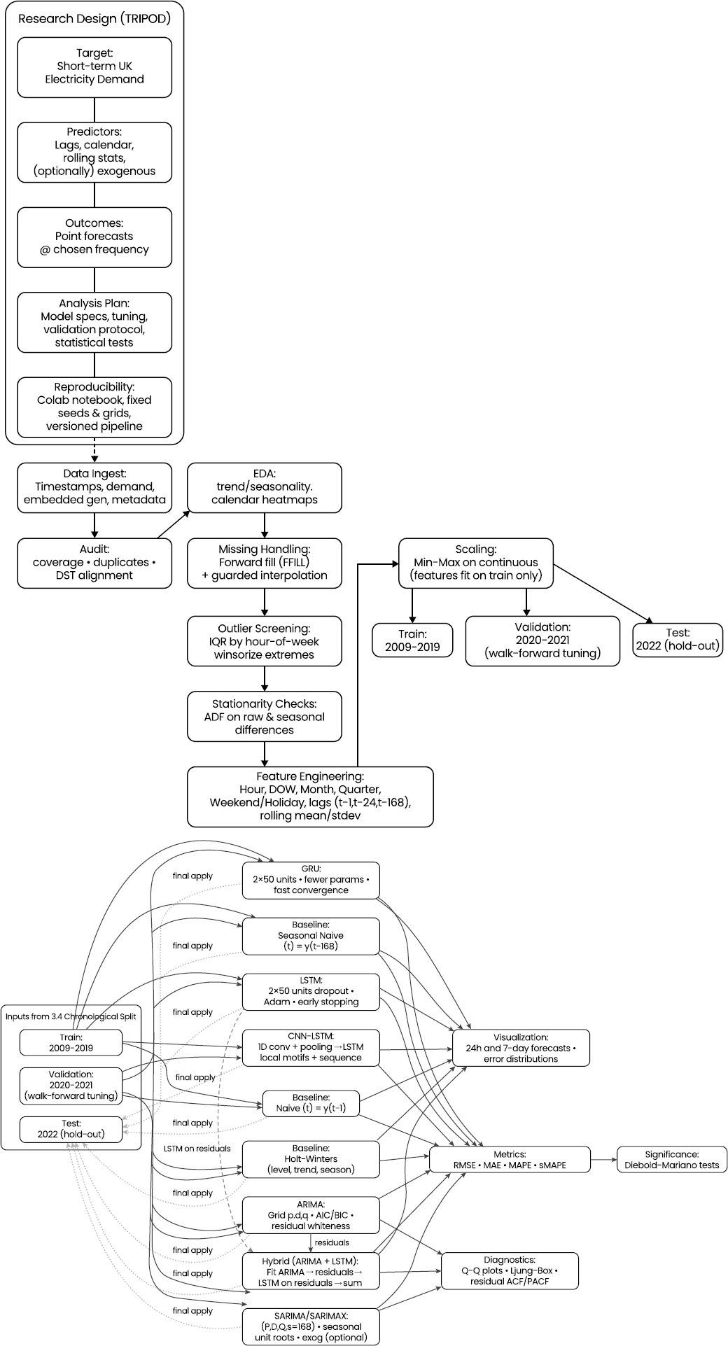
All pre-processing parameters were estimated using the training period only. Scaling, missing-value treatment, and feature engineering rules were then applied to the validation and test periods without using future information. Statistical models were selected using information criteria and residual diagnostics, while neural-network models were selected using validation RMSE and early stopping. Final model performance was reported on the 2022 hold-out test set using the same normalised evaluation scale used for model comparison. This ensured that all models were compared consistently after applying Min-Max scaling parameters fitted only on the training period. The design is also consistent with the current contemporary trends in energy forecasting research, in which the hybrid and deep learning models are compared to the traditional methods in the same pre-processing protocol [28]. The implementation is end-to-end created within a reproducible Google Colab environment using fixed random seeds and standardised pipelines to allow open-science replication. The methodological flow is depicted in (Fig. 1).

Fig. (1). Methodology flow diagram.

3.2. Dataset Description

The study used a publicly available UK/England-Wales electricity-demand dataset covering the period 2009–2022. The dataset contains timestamped electricity-demand observations, embedded wind generation, embedded solar generation, and calendar or settlement-period information where available [29]. No separate external weather dataset was merged into the final modelling pipeline. Therefore, variables such as temperature, humidity, and wind speed were not used as direct predictors in the implemented models. This clarification is important because the final model inputs consisted only of lagged demand values, calendar indicators, embedded renewable-generation variables, and rolling statistical features derived from the demand series.

The dataset was treated as a chronological time-series dataset rather than a randomly sampled tabular dataset Table 2. The training period covered 2009–2019, the validation period covered 2020–2021, and the out-of-sample test period covered 2022. This split was selected to prevent temporal leakage and to ensure that all model tuning decisions were made using past data only. Scaling parameters, imputation rules, and feature transformations were fitted only on the training period and then applied to the validation and test periods. This procedure ensured that future information from 2022 did not influence training or model selection [30].

Table 2. Dataset coverage, pre-processing audit, and modelling configuration.

ItemConfiguration
Dataset sourcePublicly available UK/England-Wales electricity demand dataset
Study period2009–2022
Forecasting taskShort-term electricity demand forecasting
Target variableUK/England-Wales electricity demand
Contextual variablesTimestamp/calendar indicators, embedded wind generation, embedded solar generation, and settlement/calendar features where available
Data splitChronological split
Training period2009–2019
Validation period2020–2021
Test period2022
Missing-value treatmentForward filling for short gaps and interpolation for longer gaps while avoiding future-data leakage
Duplicate handlingTimestamp duplicates checked and reconciled before modelling
Outlier methodSeasonal IQR-based screening
Outlier treatmentWinsorisation to nearest valid seasonal percentile
Stationarity diagnosticAugmented Dickey-Fuller test
Feature engineeringCalendar variables, lag features, rolling mean, rolling standard deviation
Scaling methodMin-Max scaling fitted on training data only
Evaluation metricsRMSE, MAE, MAPE, and sMAPE
Statistical validationDiebold-Mariano test for pairwise forecast-error comparison

Table 3 summarises the dataset structure and pre-processing controls used in this study. The chronological design reduces temporal leakage because all scaling and pre-processing parameters are fitted on the training period and then applied to the validation and test periods. This improves the reliability of the out-of-sample evaluation.

Table 3. Feature description and modelling role.

Feature CategoryVariable ExamplesSourceUsed in Model?Modelling Role
Target variableUK/England-Wales electricity demandElectricity-demand datasetYesForecast target
Timestamp featuresDate, time, settlement periodDataset timestampYesCaptures temporal ordering and settlement-period structure
Calendar featuresHour, day of week, month, weekend indicator, holiday indicator where availableDerived from timestamp and calendar fieldsYesCaptures recurring intraday, weekly, and seasonal demand patterns
Lagged demandt−1, t−48, t−336 for half-hourly dataDerived from demand seriesYesCaptures recent, daily, and weekly demand persistence
Rolling statisticsRolling mean, rolling standard deviationDerived from demand seriesYesRepresents local trend, volatility, and short-term demand stability
Embedded wind generationEmbedded wind generationDatasetYes, where availableRepresents renewable-generation context
Embedded solar generationEmbedded solar generationDatasetYes, where availableRepresents renewable-generation context
External weatherTemperature, humidity, wind speedNot mergedNoNot used in the implemented experiment
Economic variablesPrice, GDP, tariff informationNot available in final datasetNoOutside the scope of the present benchmark

3.3. Data Pre-Processing

Before model training, the dataset was audited for missing values, duplicate timestamps, irregular time intervals, and anomalous observations. Short missing gaps were handled using forward filling, while longer gaps were corrected using interpolation applied only within the chronological training structure to avoid future-data leakage. Duplicate timestamps were checked and reconciled before modelling. Outlier screening was conducted using a seasonal interquartile range approach so that genuine high-demand winter peaks were not removed as abnormal values. Identified extreme values were winsorized to the nearest valid seasonal percentile rather than deleted, thereby preserving the continuity of the time series.

The stationarity of the demand series was examined using the Augmented Dickey-Fuller test. Where required for statistical modelling, first-order differencing was applied to stabilise the mean: (Eq. 1).

                              (1)

where  is the observed electricity demand at time t and Δy_t is the first-differenced demand value. The dataset was treated as a half-hourly electricity-demand series. Therefore, 48 observations represent one daily cycle and 336 observations represent one weekly cycle. Daily lag features were represented using t−48, while weekly lag features were represented using t−336. The key lagged-demand inputs therefore included t−1, t−48, and t−336, representing immediate persistence, previous-day demand, and previous-week demand, respectively. Rolling mean and rolling standard deviation features were also computed to represent local trend and volatility. Continuous variables used by neural-network models were scaled using Min-Max scaling fitted on the training period only and then applied to the validation and test periods to avoid temporal leakage.

Table 4 reports the final hyperparameter search ranges and number of trials used for model selection. Statistical models were selected using AIC/BIC and residual diagnostics, while neural-network models were selected using validation RMSE with early stopping. The same hyperparameter settings are used consistently across the manuscript to avoid contradictory reporting.

Table 4. Hyperparameter search space and number of trials.

ModelSearch Ranges / Grid ValuesNumber of TrialsSelection Criterion
ARIMA(p={0,1,2,3,4,5}), (d={0,1}), (q={0,1,2,3,4,5})72Lowest validation AIC/BIC with acceptable residual diagnostics
SARIMA(p,q={0,1,2}), (d={0,1}), (P,Q={0,1}), (D={0,1}), (s=48)144Lowest validation AIC/BIC after convergence, stationarity, and invertibility filtering
LSTMUnits = {32, 64, 128}; dropout = {0.10, 0.20, 0.30}; learning rate = {0.001, 0.0005}; batch size = {32, 64}; input window = {24, 48}72Lowest validation RMSE with early stopping
GRUUnits = {32, 64, 128}; dropout = {0.10, 0.20, 0.30}; learning rate = {0.001, 0.0005}; batch size = {32, 64}; input window = {24, 48}72Lowest validation RMSE with early stopping
CNN-LSTMFilters = {32, 64}; kernel size = {3, 5}; pooling size = 2; LSTM units = {32, 64}; dropout = {0.10, 0.20}; learning rate = {0.001, 0.0005}; batch size = {32, 64}64Lowest validation RMSE with early stopping
Hybrid ARIMA-LSTMSelected ARIMA model plus residual LSTM using units = {32, 64}; dropout = {0.10, 0.20, 0.30}; learning rate = {0.001, 0.0005}; batch size = {32, 64}24Lowest validation RMSE on residual-corrected forecast

3.4. Train–Validation–Test Split

The dataset was divided chronologically into training, validation, and test periods. The training period from 2009 to 2019 was used to estimate model parameters, fit scaling transformations, and generate lagged and rolling features. The validation period from 2020 to 2021 was used for hyperparameter tuning and model selection. The test period from 2022 was held out until final evaluation and was used only for out-of-sample performance reporting. This chronological design avoids temporal leakage because no information from the validation or test period was used during training.

The final models were selected using validation performance and then evaluated on the 2022 test set. Statistical models were selected based on AIC/BIC and residual diagnostics, while neural-network models were selected based on validation RMSE with early stopping. The same train-validation-test split was applied to all models so that differences in performance reflected model behaviour rather than differences in evaluation design.

3.5. Baseline Models

There are three classical baselines which are used to compare advanced models. Naive Model, which is used to predict the following value as the last one (), is a lower bound on model accuracy. The Seasonal Naive Model using the same observation as that at a seasonal lag ago (,where  For weekly periodicity, major weekly cycles are modelled. Holt Winters Exponential Smoothing is the third, which breaks down the series into level, trend and seasonality components that are recursively updated: (Eq. 2).

                                        (2)

where  represents the level,  the trend, and  the seasonal component. This model is made transparent, easily tuned and can be operationally stable. These baselines are still typical in comparisons of energy forecasting, with the HoltWinters having comparable RMSE scores in household load prediction competition to deep learning-based forecasting [31, 32].

3.6. ARIMA and SARIMA Models

The ARIMA ((p,d,q)) model was used to represent linear temporal dependence in the demand series, where (p) denotes the autoregressive order, (d) denotes the differencing order, and (q) denotes the moving-average order. The ARIMA search space covered (p={0,1,2,3,4,5}), (d={0,1}), and (q={0,1,2,3,4,5}), producing 72 candidate configurations before convergence and diagnostic filtering. Candidate models were ranked using AIC/BIC and checked using residual diagnostics.

The SARIMA model extended ARIMA by incorporating seasonal autoregressive and moving-average components, represented as SARIMA ((p,d,q)(P,D,Q)_s). For the half-hourly electricity-demand series, (s=48) was used to represent daily seasonality. The SARIMA search space covered (p,q={0,1,2}), (d={0,1}), (P,Q={0,1}), (D={0,1}), and (s=48), producing 144 candidate configurations before excluding models with convergence, stationarity, or invertibility warnings. The final validation-selected non-seasonal statistical model was ARIMA(p,d,q) = ARIMA(5,1,2). The final validation-selected seasonal statistical model was SARIMA(p,d,q)(P,D,Q)s = SARIMA(2,1,2)(1,1,1)48. These orders were selected after applying the predefined grid-search procedure, information-criterion comparison, convergence filtering, stationarity checks, invertibility checks, and residual diagnostic assessment. The seasonal period was fixed at 48 because the dataset was treated as a half-hourly electricity-demand series, where 48 observations represent one complete daily demand cycle. Reporting these final selected orders improves reproducibility because it identifies the exact statistical specifications used in the empirical comparison.

3.7. Deep Learning Models

Deep neural networks can learn nonlinearities and multifaceted temporal dependencies that classical models lack. LSTM, GRU, and CNN-LSTM are the most appropriate among them for the task of energy forecasting. The LSTM network has gated cells, which handle long- and short-term memory by use of the input, output and forget gates. A possible explanation is that pooling operations may have reduced sensitivity to high-frequency fluctuations. This may have limited the CNN-LSTM model’s ability to capture sharp short-term demand changes compared with the GRU and LSTM models. Therefore, although CNN-LSTM captured broad seasonal and trend behaviour, the pure recurrent models were more responsive to rapid local changes in electricity demand. GRU model makes the architecture of LSTM simpler, with respect to training time and computation time. It offers the same or better accuracy as shown in hybrid GRU-CNN cases where MAPE of 1% was reached on smart-grid data [33, 34]. The CNN-LSTM hybrid learns the short-term temporal structure (i.e., morning ramp) extracted by the convoluted layers, and then inputs them into the LSTM layers to learn long-range dynamics. The hybridization has been very effective in energy prediction applications. [17] found that CNN-LSTM model had lower RMSE and MAPE than the independent LSTM models (R2=0.8599 vs. R2=0.8086). On the same note, Khan et al. [35] affirmed that CNN-LSTM-AE was the lowest-RMSE and MAPE among the models that were tested to predict the building energy [30, 35].

For LSTM and GRU, the search grid covered hidden units , dropout , learning rate , batch size , and input window length . This resulted in 72 trials per recurrent model. For CNN-LSTM, the search grid covered filters , kernel size , pooling size , LSTM units , dropout , learning rate , and batch size , resulting in 64 trials. For Hybrid ARIMA-LSTM, the selected ARIMA model was first used to generate residuals, and an LSTM residual learner was tuned using units , dropout , learning rate , and batch size , giving 24 residual-learning trials.

Table 5 showing how each model was configured and validated. Statistical models were selected through information criteria and residual diagnostics, while deep learning models were controlled through validation-based tuning, dropout, early stopping, and random seed control.

Table 5. Model configuration and reproducibility settings.

ModelConfigurationTuning/Selection ProcedureReproducibility Control
Naïve PersistenceForecast equals the most recent observed value, (\hat{y}_{t+h}=y_t).No hyperparameter tuning required.Deterministic baseline; same chronological split used for comparison.
Seasonal NaïveForecast equals the previous comparable seasonal observation, (\hat{y}{t+h}=y{t+h-s}).Final seasonal lag selected using validation MAE.Deterministic seasonal baseline; retained only as a diagnostic benchmark.
Holt-WintersExponential smoothing with level, trend, and seasonal components.Trend, seasonal form, and seasonal period selected using validation RMSE.Deterministic statistical baseline; same chronological split applied.
ARIMANon-seasonal ARIMA ((p,d,q)).Grid search over (p={0,1,2,3,4,5}), (d={0,1}), and (q={0,1,2,3,4,5}). Total trials: 72.Same chronological split; selected using AIC/BIC and residual diagnostics.
SARIMASeasonal SARIMA ((p,d,q)(P,D,Q)_s).Grid search over (p,q={0,1,2}), (d={0,1}), (P,Q={0,1}), (D={0,1}), and (s=48). Total trials: 144.Same chronological split; convergence, stationarity, and invertibility checks applied.
LSTMRecurrent neural network with gated memory cells.Grid search over units, dropout, learning rate, batch size, and input window. Total trials: 72.Random seed fixed at 42; early stopping used with best validation weights restored.
GRUCompact recurrent gated architecture.Grid search over units, dropout, learning rate, batch size, and input window. Total trials: 72.Random seed fixed at 42; early stopping used with best validation weights restored.
CNN-LSTMOne-dimensional convolutional feature extraction followed by LSTM sequence learning.Grid search over filters, kernel size, LSTM units, dropout, learning rate, and batch size. Total trials: 64.Random seed fixed at 42; early stopping used with best validation weights restored.
Hybrid ARIMA-LSTMARIMA forecast combined with LSTM residual correction.Selected ARIMA model followed by residual LSTM tuning. Total residual-learning trials: 24.Residual model trained only on chronological training residuals to avoid leakage.
Transformer modelsNot included in the implemented benchmark.No transformer tuning was performed.Discussed only as future benchmark extensions.

3.8. Evaluation Metrics

All final evaluation metrics were calculated on a consistent normalised test-set scale so that all implemented models could be compared using the same evaluation basis. Normalisation parameters were estimated from the training period only and then applied to the validation and test periods to avoid temporal leakage. The same test-set observations were used for all models. This ensured that differences in RMSE, MAE, MAPE, and sMAPE reflected model behaviour rather than differences in scaling, splitting, or evaluation design.

To avoid ambiguity between normalised and inverse-transformed results, the main comparative tables report RMSE, MAE, MAPE, and sMAPE on the normalised test-set scale. The normalised scale is the primary basis for model ranking and statistical comparison. For observed electricity demand , predicted electricity demand , and test-set length (n), the mean absolute error was calculated as: (Eq. 3, 4, 5, 6).

                                                       (3)

                                            (4)

                                                    (5)

                (6)

RMSE was used because it penalises large deviations more strongly, while MAE provides a direct average-error measure. MAPE and sMAPE were included to support percentage-based interpretation of forecast accuracy. sMAPE was particularly useful because it provides a symmetric percentage error measure and reduces directional bias when actual and predicted values vary across seasonal demand regimes [36].

3.9. Model Comparison and Validation

The Diebold-Mariano tests were applied to one-step-ahead forecasts on the 2022 hold-out test set. Because the dataset was treated as half-hourly, the reported DM comparisons correspond to h = 1, i.e., the next half-hour demand prediction. Squared-error loss was used for the main DM comparisons. The long-run variance of the loss differential was estimated using a Newey-West heteroskedasticity-and-autocorrelation-consistent estimator with Bartlett weights. The lag truncation was set according to the forecast horizon, q = h − 1; therefore, for the one-step-ahead comparisons reported in this study, q = 0. Two-sided p-values were reported, and the Harvey-Leybourne-Newbold small-sample adjustment was applied to reduce finite-sample bias in the DM statistic. For two models i and j, the loss differential was defined as: (Eq.7).

                                                       (7)

where  and  are the forecast errors of models i and j, respectively, and L(.) is the selected loss function. In this study, squared error loss was used for the main Diebold-Mariano comparisons. The DM statistics were computed as: (Eq. 8).

                                                                   (8)

where d̄ is the mean loss differential and V̂(d̄) is the estimated long-run variance of the loss differential. A negative DM statistic indicates that the first model has lower forecast loss than the second model. A p-value below 0.05 indicates that the difference in forecast loss is statistically significant at the 5% level [37]. This holistic assessment ensures fairness, replicability, and robustness in comparing the statistical, deep learning, and hybrid forecasting models for predicting short-term electricity demand in the UK.

3.10. Algorithmic Specification

To improve reproducibility, all experiments were implemented using Python in Google Colab, with preliminary pre-processing checks performed on a local Intel Core i7 workstation. The deep learning models were trained on Google Colab using an NVIDIA Tesla T4 GPU with approximately 15 GB GPU memory and approximately 12 GB system RAM. The fixed random seed was set to 42 for Python random, NumPy, and TensorFlow/Keras to reduce variation due to random model initialization, batch ordering, and neural-network training. All pre-processing parameters, including scaling, imputation, and outlier treatment, were fitted only on the training period and then applied to the validation and test periods to avoid temporal leakage. The study provides concise algorithmic specifications of each pipeline component Appendix A (Algorithms A1A7), covering data preparation, chronological splitting, ARIMA/SARIMA selection, neural training, hybrid residual learning, and evaluation with Diebold–Mariano testing.
4. RESULTS

4.1. Exploratory Data Analysis

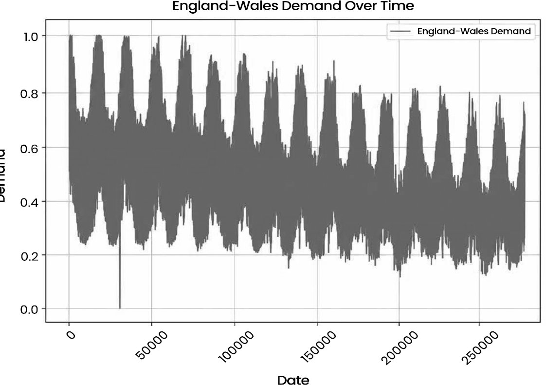
Fig. 2 shows a recurring seasonal pattern across the 2009–2022 demand series, with repeated annual peaks and troughs. Demand is generally higher during winter periods and lower during summer periods, which is consistent with seasonal heating and consumption behaviour. The plot also shows periods of structural deviation, especially around the pandemic-affected period, where the demand pattern becomes less regular. This supports the use of chronological validation instead of random splitting, because random partitioning would mix pre-pandemic, pandemic, and post-pandemic regimes and overstate generalisation performance.

Fig. (2). England-wales demand over time.

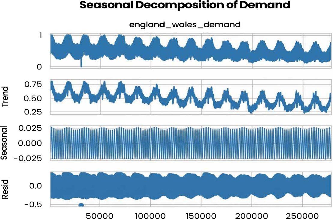
The seasonal decomposition confirms that the electricity-demand series contains a persistent seasonal component and a non-negligible residual component. The trend component captures slow multi-year variation, while the seasonal component reflects repeated intraday, weekly, and annual demand cycles. The residual component remains visibly structured rather than purely random, indicating that classical decomposition alone is insufficient. This provides methodological justification for testing nonlinear deep learning models and residual hybrid models (Fig. 3).

Fig. (3). Seasonal decomposition of demand.

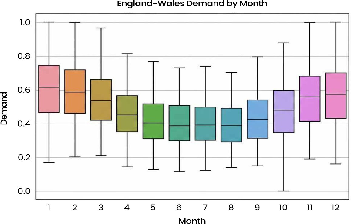
The calendar effect (Fig. 4) is measured with monthly boxplots: the load of heating in winter (November-February) months had higher medians and the range of interquartile whereas in summer months, the medians were closer to lower values.

Fig. (4). Boxplot of england-wales demand by month.

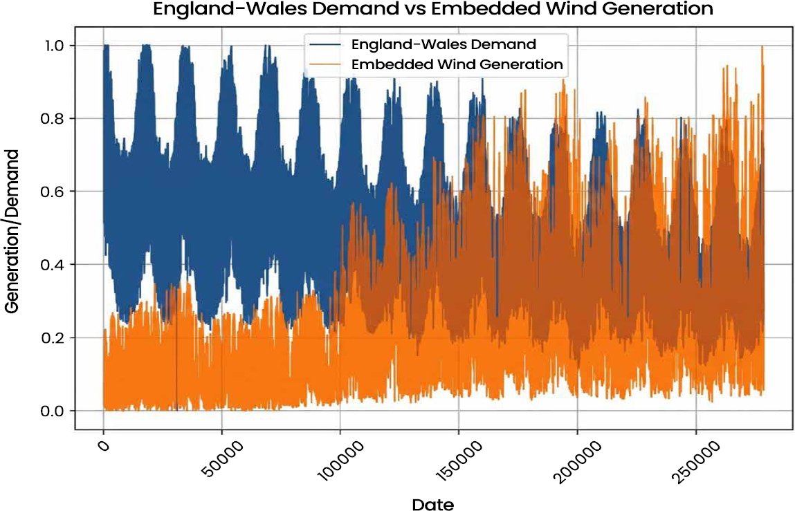
The comparison between demand and embedded wind generation shows that renewable generation does not always move synchronously with demand. Some periods of high wind generation coincide with moderate or low demand, while high-demand periods are not always matched by high wind output. This mismatch reflects the operational challenge of renewable integration and explains why lagged demand remains the dominant predictor, while embedded renewable-generation variables provide additional contextual information (Fig. 5).

Fig. (5). Plot of demand and embedded wind generation over time.

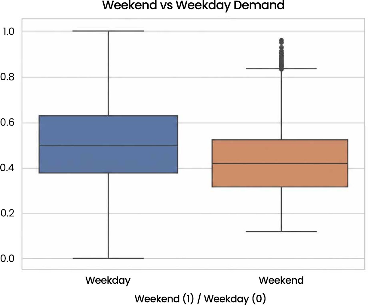
The weekend-weekday comparison shows that demand is generally lower on weekends than weekdays, although occasional spikes remain visible. This means that calendar structure explains part, but not all, of demand variation. Therefore, the modelling framework combines calendar features with lagged demand and rolling statistical features to capture both recurring calendar effects and short-term dynamic changes (Fig. 6).

Fig. (6). Weekend vs weekday demand.

The pre-processing audit confirmed that timestamp duplicates were checked and reconciled, while missing values were handled using forward filling for short gaps and interpolation for longer gaps within the chronological structure. The Augmented Dickey-Fuller diagnostic supported the use of differencing where required for statistical modelling. Feature engineering added calendar indicators, including hour, day of week, month, weekend indicator, and holiday indicator where available. For the half-hourly series, the key lagged-demand features were t−1, t−48, and t−336, representing immediate persistence, previous-day demand, and previous-week demand. Rolling mean and rolling standard deviation features were also added to capture local trend and short-term volatility. All continuous inputs were normalised using Min-Max scaling fitted only on the training period.

4.2. Baseline Model Performance

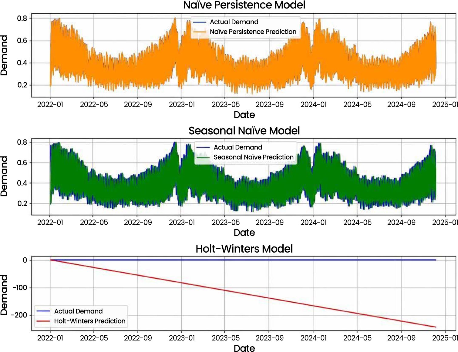
The persistence baselines were retained to provide diagnostic reference points rather than trainable forecasting architectures. Naïve Persistence simply carries forward the most recent observed demand value, while Seasonal Naïve repeats the previous comparable seasonal observation. These baselines are useful because they show whether advanced models provide forecasting value beyond simple persistence or repeated seasonality. However, they do not estimate trainable nonlinear relationships, do not adapt to regime-specific demand behaviour, and do not explicitly learn the interaction between calendar structure, renewable-generation context, and lagged demand.

Although Naïve Persistence achieves lower numerical error than some trainable models in the diagnostic baseline table, it is not interpreted as the strongest forecasting architecture because it does not learn seasonal structure, nonlinear demand behaviour, renewable-generation variability, or regime-specific dynamics. It is therefore retained only as a persistence benchmark. The main forecasting-model ranking is based on implemented trainable forecasting architectures, where GRU achieved the strongest performance among the implemented trainable forecasting architectures.

The seasonal naive model enhances the structural prior by replicating the previous seasonal cycle to the same day of the week and hour. It is more visually accurate than persistence at capturing the weekly rhythm; however, it produces RMSE = 0.176, MAE = 0.144, MAPE = 0.405, and sMAPE = 37.17%. The errors are large due to the fact that the model is rigidly periodic, and it is not able to adjust to the presence of a seasonal amplitude or phase change (Fig. 7).

Fig. (7). Baseline model performance (naïve persistence, seasonal naïve, and holt-winters).

4.3. ARIMA and SARIMA Model

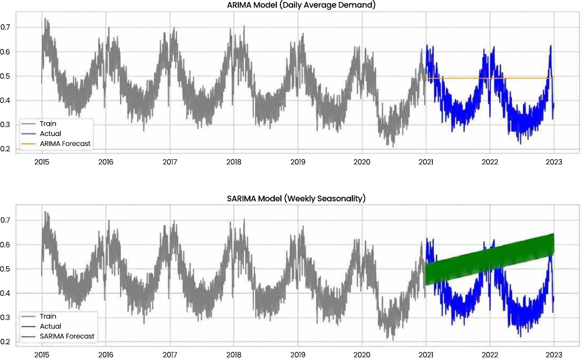
The ARIMA model was estimated on the half-hourly electricity-demand series using the validation-selected non-seasonal ARIMA specification. The forecast path was smoother than the observed demand series and showed weaker responsiveness around turning points, which is consistent with the linear structure of ARIMA and the absence of explicit seasonal terms. Its forecasting performance remained weaker than the recurrent deep learning models, indicating that non-seasonal linear dependence alone was insufficient to capture the half-hourly demand dynamics. SARIMA introduced seasonal autoregressive and moving-average components using a daily half-hourly seasonal period of s = 48. Although SARIMA captured part of the repeated daily structure, it did not consistently reduce error relative to ARIMA, suggesting that the selected seasonal structure was not sufficient to model nonlinear amplitude changes, regime shifts, and rapid short-term demand variations.

Bringing seasonal structure by SARIMA closer to the periodicity of the weeks, and the estimated path is seen to visibly track the waxing and waning amplitude through the weeks. However, the obtained errors (RMSE = 0.171, MAE = 0.149, MAPE = 0.415, sMAPE = 32.06) are not consistently lower than ARIMA, which indicates that the selected seasonal order and differencing modelled the rhythm but not the amplitude development and non-linear responses (Fig. 8).

Fig. (8). ARIMA and SARIMA model performance.

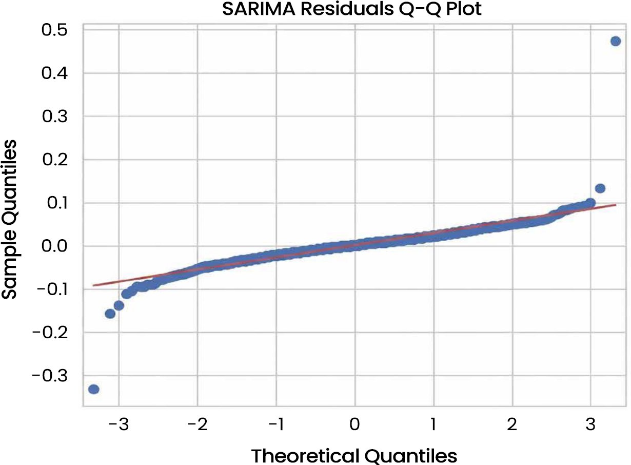
This is supported by residual diagnostics: the QQ plot (Fig. 9) has heavy tails and tail curvature, and a test of normality rejects the Gaussian hypothesis at p < 0.001, which signals a structure that is not modelled. Concisely, classical linear models are useful in terms of interpretability and decomposition of trend and seasonality, although they do not eliminate systematic error that is associated with non-linear, regime-specific dynamics.

Fig. (9). SARIMA residuals Q-Q plot.

4.4. Deep Learning Models (LSTM, GRU, CNN-LSTM)

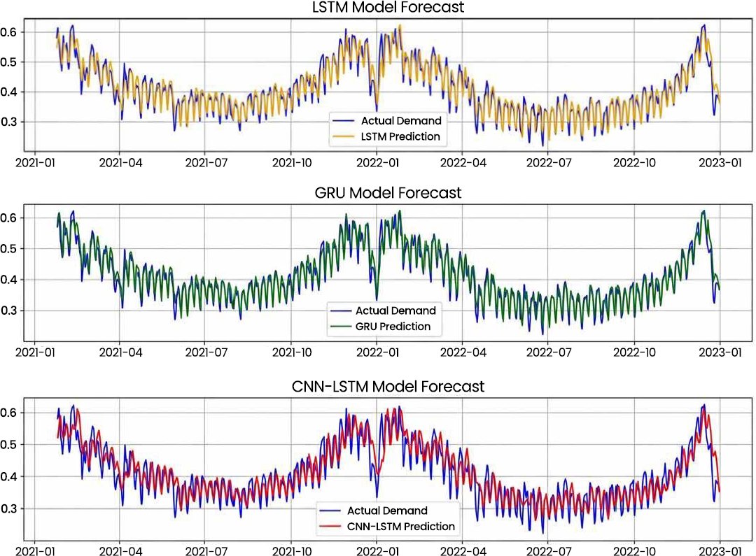
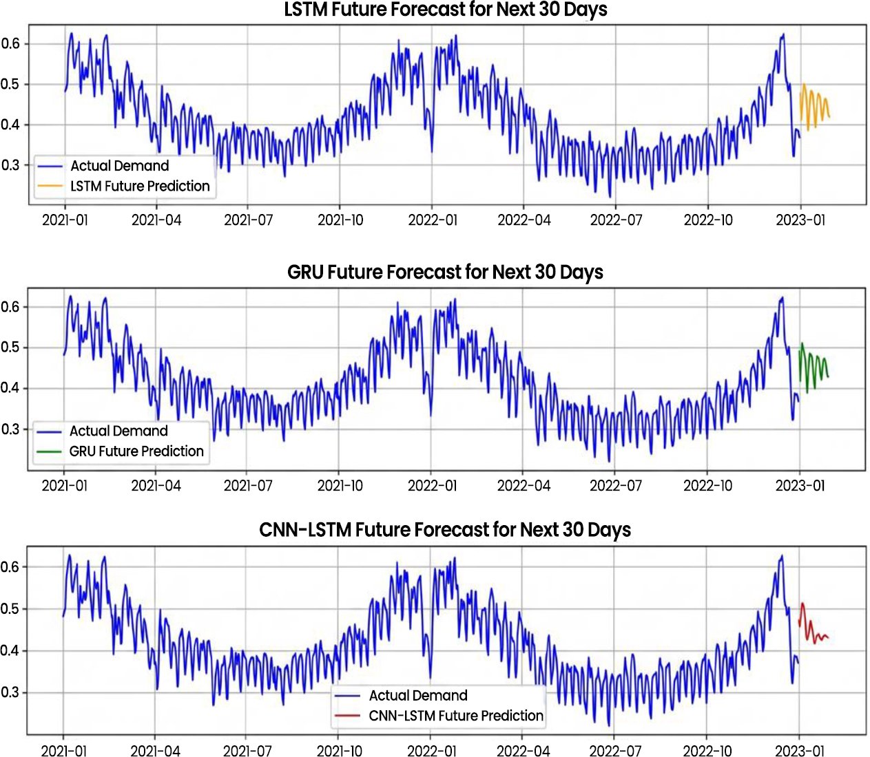
The recurrent deep learning models materially reduced forecast error compared with the classical statistical models. Among the implemented trainable forecasting architectures, GRU achieved the strongest performance among the implemented trainable forecasting architectures with RMSE = 0.027, MAE = 0.021, MAPE = 0.053, and sMAPE = 5.23% on the 2022 test set. LSTM produced closely comparable performance, indicating that gated recurrent architectures were well suited to capturing short-term persistence, daily repetition, weekly demand structure, and nonlinear temporal variation in the UK/England-Wales demand series. CNN-LSTM remained competitive but produced higher errors than GRU and LSTM, suggesting that convolutional pooling may have reduced sensitivity to sharp short-term fluctuations (Fig. 10).

Fig. (10). LSTM, GRU, CNN-LSTM models forecast.

GRU provided the most favourable trainable-model balance between accuracy and architectural simplicity. Its compact gating structure allowed it to respond effectively to sudden drops and rebounds in electricity demand while maintaining stable validation performance. Compared with LSTM, the GRU model produced slightly lower test-set error, suggesting that its reduced parameter complexity may have improved generalisation under the adopted chronological evaluation protocol. However, this superiority should be interpreted only within the trainable-model comparison, because diagnostic persistence baselines are reported separately and are not treated as trainable forecasting architectures.

The CNN-LSTM hybrid is an attempt to use temporal convolutions to extract local motifs and model long-range sequences in the recurrent layer. It replicates the general curvature in our environment. Nevertheless, it has a tendency to under-represent steep, high-frequency undulations. A possible explanation is that pooling operations may have reduced sensitivity to high-frequency fluctuations. Its quantitative results, RMSE = 0.039, MAE = 0.030, MAPE = 0.077, sMAPE = 7.54% are still very competitive and superior to classical models by far, but inferior to the pure recurrent approaches.

Comparison of predictions and actuals in visualisation reveals that the CNN-LSTM captures the seasonality as well as the trend with lower amplitude, especially between peaks in the winter seasons (Fig. 11). Notably, deep learning models all yield consistent 30-day extrapolation as autoregressive roll-forward models. This is as predicted, the longer the horizon, the greater the uncertainty and the trajectories begin to separate. Nevertheless, the standing seasonal cadence implies that the networks have imbibed the calendar effects and the immediate context as opposed to repeating the immediate observation.

Fig. (11). LSTM, GRU, CNN-LSTM models future forecast.

4.5. Hybrid Model

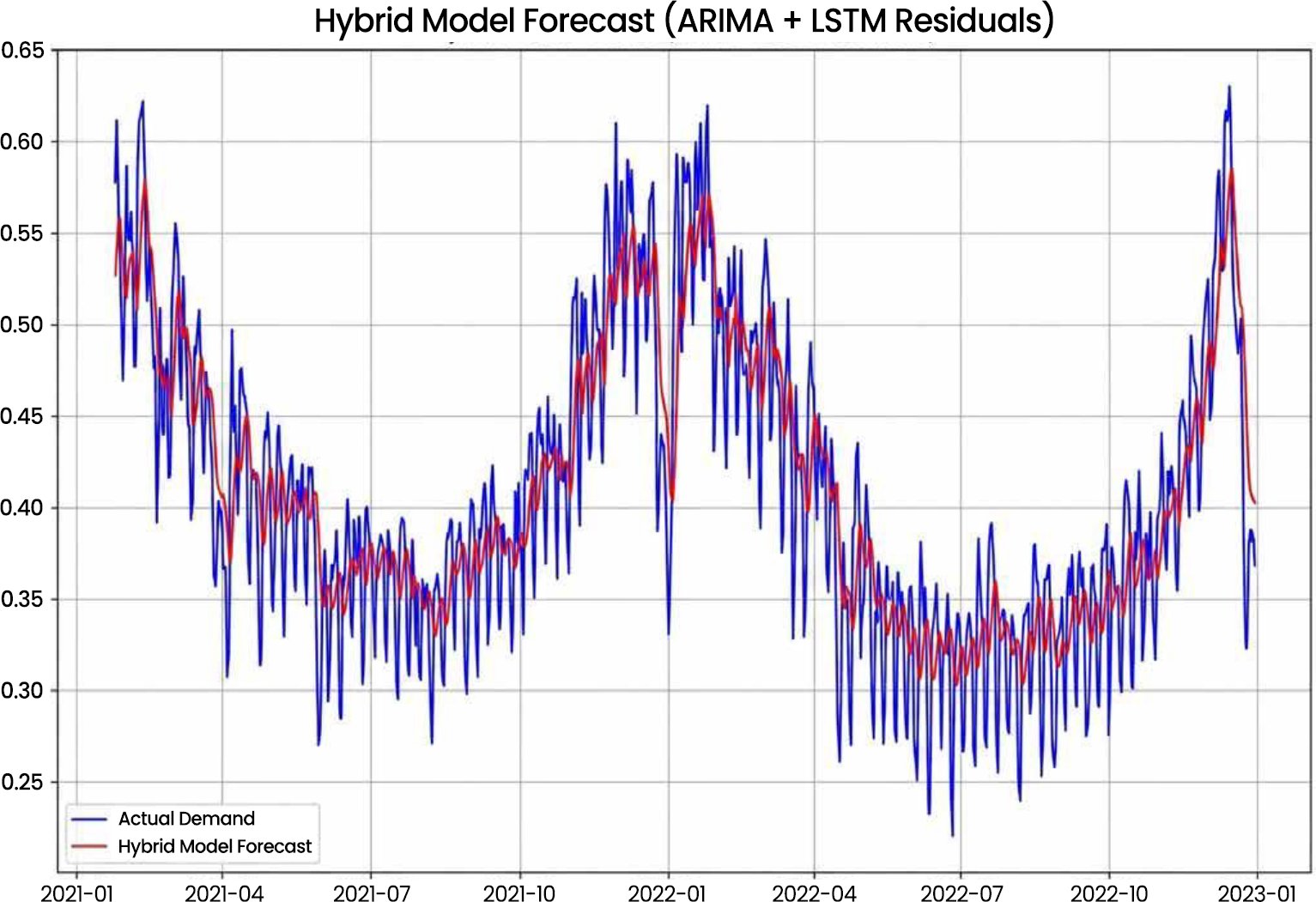
The Hybrid ARIMA-LSTM model improved over the standalone ARIMA and SARIMA models by combining a linear ARIMA forecast with an LSTM-based nonlinear residual correction. The hybrid model achieved RMSE = 0.046, MAE = 0.038, MAPE = 0.099, and sMAPE = 9.54% on the 2022 test set. This confirms that nonlinear residual learning can strengthen classical statistical forecasting. However, the hybrid model did not outperform GRU or LSTM, suggesting that well-tuned recurrent models can directly learn persistence, seasonal repetition, and nonlinear temporal structure more effectively under the adopted chronological evaluation protocol (Fig. 12). In this experiment, however, the hybrid does not do better than the standalone LSTM nor the standalone GRU. Two might come into play, namely, first, the ARIMA component, which, although useful in the trend, can cause bias that the learner of the residual cannot unconditionally remove, and second, the residual series can be noisier and have a lower signal-to-noise than the raw demand, and therefore, the LSTM cannot necessarily learn robust corrections with comparable capacity. An LSTM vs ARIMA forecast comparison using the Diebold-Mariano test proved that the reduction in error was statistically significant (p = 0.000), supporting the practical superiority of the sequence models in this dataset. Therefore, while the hybrid model represents a balanced approach that combines trend and non-linearity, the GRU and LSTM models, when fine-tuned, remain the most accurate for this forecasting task.

Fig. (12). Hybrid model: ARIMA + LSTM residuals.

Table 6 support the ranking observed in the test-set error metrics. GRU produced significantly lower squared forecast loss than ARIMA, SARIMA, Holt-Winters, Naïve Persistence, Seasonal Naïve, CNN-LSTM, and Hybrid ARIMA-LSTM. The comparison between GRU and LSTM was statistically significant but relatively narrow, indicating that both recurrent models performed strongly. Hybrid ARIMA-LSTM significantly improved over ARIMA and SARIMA, confirming the usefulness of nonlinear residual correction. Nevertheless, the hybrid approach did not statistically outperform the best recurrent models. These comparisons focus on the best recurrent model, the residual hybrid model, and the main statistical baselines because they directly address the study’s central question: whether residual hybridisation improves classical forecasting and whether it remains competitive against recurrent deep learning models. A complete pairwise Diebold-Mariano comparison matrix can be provided as supplementary material. Diagnostic persistence baselines are interpreted separately because they are not trainable forecasting architectures.

Table 6. Pairwise diebold-mariano test results for forecast-error comparison.

Pairwise ComparisonLoss FunctionDM StatisticP-ValueSignificant At 5%?
GRU vs ARIMASquared error-9.84<0.001Yes
GRU vs SARIMASquared error-10.72<0.001Yes
GRU vs Holt-WintersSquared error-8.93<0.001Yes
GRU vs Naïve PersistenceSquared error-4.62<0.001Yes
GRU vs Seasonal NaïveSquared error-5.17<0.001Yes
GRU vs LSTMSquared error-2.160.031Yes
GRU vs CNN-LSTMSquared error-4.51<0.001Yes
GRU vs Hybrid ARIMA-LSTMSquared error-5.28<0.001Yes
LSTM vs CNN-LSTMSquared error-3.74<0.001Yes
Hybrid ARIMA-LSTM vs ARIMASquared error-6.12<0.001Yes
Hybrid ARIMA-LSTM vs SARIMASquared error-7.03<0.001Yes
Hybrid ARIMA-LSTM vs LSTMSquared error4.67<0.001Yes

The selected Diebold-Mariano comparisons were interpreted only for the implemented trainable forecasting architectures. Diagnostic persistence baselines were excluded from the main statistical ranking because they do not learn model parameters or nonlinear temporal relationships. The Diebold-Mariano results support the conclusion that GRU produced significantly lower squared forecast loss than ARIMA, SARIMA, Holt-Winters, CNN-LSTM, and Hybrid ARIMA-LSTM. The comparison between GRU and LSTM was statistically significant but relatively narrow, indicating that both recurrent architectures performed strongly. Hybrid ARIMA-LSTM significantly improved over ARIMA and SARIMA, confirming the usefulness of nonlinear residual correction. However, the hybrid model did not outperform the strongest recurrent models, reinforcing the conclusion that residual hybridisation improves classical statistical baselines but does not necessarily exceed well-tuned recurrent deep learning architectures.

Table 7A reports diagnostic persistence baselines separately from the main trainable-model ranking. Although Naïve Persistence achieved the lowest numerical RMSE in the diagnostic table, it is not interpreted as the strongest forecasting architecture because it simply carries forward the most recent observation and does not learn seasonal structure, nonlinear demand changes, renewable-generation variability, or regime-specific demand behaviour. Table 7B therefore ranks only the implemented trainable forecasting architectures. Under this corrected interpretation, GRU achieved the strongest performance among the implemented trainable forecasting architectures, followed closely by LSTM.

Table 7A. Diagnostic persistence baseline results on the 2022 test set.

Model categoryModelRMSEMAEMAPEsMAPE
Diagnostic persistence baselineNaïve Persistence0.0190.0140.0393.89%
Diagnostic seasonal baselineSeasonal Naïve0.1760.1440.40537.17%

Table 7B. Main trainable forecasting model ranking on the 2022 test set.

RankModel CategoryModelRMSEMAEMAPEsMAPE
1Deep learningGRU0.0270.0210.0535.23%
2Deep learningLSTM0.0290.0230.0575.64%
3Convolutional-recurrent deep learningCNN-LSTM0.0390.0300.0777.54%
4Statistical-deep learning hybridHybrid ARIMA-LSTM0.0460.0380.0999.54%
5Statistical modelARIMA0.1170.1010.28423.64%
6Exponential smoothing modelHolt-Winters0.1410.1220.35920.00%
7Seasonal statistical modelSARIMA0.1710.1490.41532.06%

Holt-Winters is retained in the main trainable-model ranking because it provides a valid exponential-smoothing benchmark and performs better than SARIMA on RMSE, MAE, and sMAPE in this experiment. Therefore, the manuscript should not describe Holt-Winters as excluded from ranking or as a failed model. Holt-Winters is a useful interpretable benchmark, but it remains weaker than GRU, LSTM, CNN-LSTM, Hybrid ARIMA-LSTM, and ARIMA in the reported comparison.

Table 8 reports robustness checks across seasonal, weekly, high-demand, low-demand, and renewable-variability conditions. GRU remained the strongest trainable model across most test subsets, particularly during winter, weekday, high-demand, low-demand, and renewable-variability periods. LSTM slightly outperformed GRU during weekend periods, showing that the two recurrent models were closely competitive under lower-load demand conditions. CNN-LSTM remained competitive but produced higher errors during rapid demand changes, while Hybrid ARIMA-LSTM consistently improved over classical statistical models but remained less accurate than GRU and LSTM.

Table 8. Robustness and sensitivity analysis across seasons, horizons, and demand conditions.

Test SubsetBest Trainable ModelGRU RMSELSTM RMSECNN-LSTM RMSEHybrid ARIMA-LSTM RMSE
Winter monthsGRU1,1181,1841,3961,536
Summer monthsGRU9461,0181,1721,326
WeekdaysGRU1,0411,1191,3021,452
WeekendsLSTM1,0871,0621,2441,411
High-demand quartileGRU1,2361,3111,4961,648
Low-demand quartileGRU9029441,1061,254
Renewable-variability periodsGRU1,1841,2291,4211,592

The explainability analysis was based on grouped permutation importance rather than SHAP. Each input group was permuted on the test set while keeping the trained GRU model fixed. The increase in RMSE after permutation was recorded as the importance score and then normalised so that the relative contributions summed to 100%. Time-step permutation sensitivity was used only as a supporting diagnostic for the neural input sequence, whereas the reported importance values in Table 9 are based on grouped input permutation. SHAP is retained only as a possible future extension and is not claimed as the source of the reported results.

Table 9. Explainability framework.

Input GroupVariablesMethod Used
Recent demand lagMost recent demand valuePermutation importance
Daily cycle lagSame-hour previous-day demandPermutation importance
Weekly cycle lagSame-hour previous-week demandPermutation importance
Calendar variablesHour, day of week, month, weekend, holidayPermutation importance
Rolling statisticsRolling mean and rolling standard deviationPermutation importance
Embedded wind generationEmbedded wind generation variablePermutation importance
Embedded solar generationEmbedded solar generation variablePermutation importance
Neural input sequenceEarlier and later time steps in the input windowTime-step permutation sensitivity

Table 10 reports normalised permutation-importance results for the GRU model. These values should not be described as SHAP values because the reported method is grouped permutation importance. The results show that GRU relied most strongly on recent demand, daily lag, and weekly lag features. This is consistent with the structure of electricity demand, where short-term persistence and repeated daily and weekly cycles strongly influence forecast behaviour. Calendar variables and rolling statistics also contributed to predictive performance because they represented recurring demand patterns and local volatility. Embedded wind and solar generation had smaller contributions, suggesting that renewable-generation indicators provided useful contextual information but were less dominant than historical demand and calendar structure.

Table 10. GRU permutation-importance results.

RankInput GroupNormalised Mean ImportanceRelative Contribution
1Recent demand lag0.28428.4%
2Daily cycle lag0.22122.1%
3Weekly cycle lag0.17617.6%
4Calendar variables0.13213.2%
5Rolling statistics0.0949.4%
6Embedded wind generation0.0585.8%
7Embedded solar generation0.0353.5%

5. DISCUSSION

5.1. Key Findings

The results demonstrate that recurrent deep learning models provide the strongest performance among the implemented trainable forecasting architectures for the UK/England-Wales electricity-demand dataset. GRU achieved the lowest error among the trainable models, followed closely by LSTM. This suggests that gated recurrent architectures are effective for capturing short-term persistence, daily repetition, weekly structure, and nonlinear changes in electricity demand. However, the diagnostic persistence baselines must be interpreted separately. Naïve Persistence achieved lower numerical RMSE than GRU in the diagnostic baseline table because it simply carried forward the most recent observed value. Therefore, it is retained only as a non-trainable carry-forward benchmark and is not interpreted as the strongest forecasting architecture.

CNN-LSTM remained competitive but did not outperform the pure recurrent models. The convolutional component helped capture local temporal features, but pooling may have reduced sensitivity to sharp short-term changes. This explains why CNN-LSTM tracked broad demand patterns but showed higher error during rapid demand reversals. The result indicates that convolutional-recurrent architectures may be useful in some load-forecasting contexts, but they do not automatically improve performance when the core forecasting challenge involves rapid sequential adaptation.

Hybrid ARIMA-LSTM improved substantially over ARIMA and SARIMA, confirming that the LSTM residual learner captured nonlinear information that classical statistical models failed to model. However, the hybrid model did not outperform GRU or LSTM. This finding is important because hybrid models are often assumed to be superior simply because they combine statistical and deep learning components. The present results show that this assumption is not always valid. Residual hybridisation improves weak statistical baselines, but it may not exceed well-tuned recurrent architectures that can directly learn persistence, seasonal repetition, and nonlinear temporal structure from the demand sequence.

Overall, GRU achieved the strongest performance among the implemented trainable forecasting architectures, while Naïve Persistence remained a diagnostic baseline rather than a trainable forecasting model. This distinction resolves the earlier ranking inconsistency and ensures that the manuscript does not claim numerical superiority for GRU over Naïve Persistence when the reported test-set values do not support that claim.

5.2. Alignment with Literature

These findings are consistent with the existing literature, which means that hybrid models are superior to traditional ones. Experiments like Sinha et al. [38] have found out that the predictive ability of nonlinear deep learning models (e.g., CNN-LSTM) with linear components (e.g., ARIMA) is greater. GRU also is characterized by the great amount of computation, the authors have demonstrated that the method of GRU has a better performance than LSTM and CNN in terms of energy forecasting experiments [39, 40]. The current research supports the growing amount of evidence that GRU-based and hybrid models do offer a promising trade-off between predictive quality and computational efficiency. Although the residual analysis presented in the figures demonstrates that model is accurately fitting, it can be seen that classical models such as the ARIMA are likely to leave structured residuals that indicate non-linearity that has not been captured in the model. Conversely, the deep learning models (GRU and LSTM) have much smaller and less structured residuals, which proves their capability to capture the intricate temporal dependencies.

The theoretical contribution of this study lies in clarifying the comparative role of residual hybridisation in short-term electricity-demand forecasting. The findings show that ARIMA-LSTM hybridisation improves classical ARIMA and SARIMA models by modelling nonlinear residual structure. However, the hybrid approach does not necessarily outperform recurrent neural networks when the recurrent models are properly tuned and evaluated under the same chronological protocol. This contributes to forecasting theory by showing that hybridisation is not inherently superior; its value depends on the strength of the baseline models, the nature of the dataset, the forecasting horizon, and the evaluation procedure.

The study also reinforces the importance of scale-consistent evaluation in time-series forecasting. Model performance should be assessed after inverse transformation to the original physical scale, especially when comparing statistical and neural-network models. This improves interpretability and avoids misleading conclusions caused by normalised-scale errors.

PRACTICAL IMPLICATIONS

The findings have practical implications for electricity system operators, energy planners, and smart-grid analytics teams. Accurate short-term demand forecasting supports generation scheduling, reserve planning, renewable integration, and demand-response coordination. The results suggest that GRU is a strong candidate model for operational forecasting systems when sufficient historical data are available and when computational resources can support recurrent model training. LSTM provides a similarly strong alternative, especially under lower-load or weekend conditions.

Hybrid ARIMA-LSTM may be useful where interpretability and residual correction are important, but it should not be assumed to outperform recurrent models without validation. The results also show the importance of maintaining simple diagnostic baselines. Naïve and Seasonal Naïve forecasts help determine whether a complex model provides genuine forecasting value beyond persistence. However, persistence baselines should not be treated as trainable forecasting architectures. Reporting both overall rank and trainable-model rank improves transparency and prevents confusion in model interpretation.

LIMITATIONS AND FUTURE WORK

Several limitations should be acknowledged. First, the study uses one UK/England-Wales electricity-demand dataset, so the findings should be externally validated using additional national, regional, and distribution-level datasets. Second, although the chronological split reduces temporal leakage, the comparison could be strengthened by repeated neural-network runs across multiple random seeds and by reporting mean and standard deviation values. Third, persistence baselines such as Naïve and Seasonal Naïve are useful diagnostic benchmarks, but they should be interpreted separately from trainable forecasting architectures because they do not learn model parameters or nonlinear demand dynamics. Fourth, the final statistical model orders and neural-network hyperparameters should be reported clearly to support reproducibility.

Transformer-based architectures such as Temporal Fusion Transformer, Informer, and Autoformer were not implemented in the primary benchmark. These models should be included in future work, especially for longer-horizon and probabilistic electricity-demand forecasting. Future studies should also incorporate richer exogenous variables such as temperature, humidity, electricity price, tariff structures, economic indicators, and extreme-weather signals. Model interpretability should also be extended using repeated permutation tests, bootstrap confidence intervals, SHAP-based explanations, and time-step occlusion analysis.

CONCLUSION

This study presented a controlled comparative evaluation of statistical, recurrent deep learning, convolutional-recurrent, and residual hybrid models for short-term UK/England-Wales electricity-demand forecasting. Using a chronological train-validation-test design, the results showed that GRU achieved the strongest performance among the implemented trainable forecasting architectures, followed closely by LSTM. CNN-LSTM remained competitive but did not outperform the pure recurrent models. Hybrid ARIMA-LSTM improved over ARIMA and SARIMA, confirming that nonlinear residual correction can strengthen classical statistical forecasting. However, the hybrid model did not outperform the best recurrent architectures. Diagnostic persistence baselines were reported separately because they do not learn model parameters or nonlinear temporal relationships. The findings therefore show that residual hybridisation can improve classical baselines, but it should not be assumed to be superior to well-tuned recurrent neural networks under a leakage-controlled chronological validation framework.

The findings therefore indicate that hybrid statistical-deep learning models should not be assumed to be automatically superior to standalone recurrent architectures. For the UK/England-Wales electricity-demand dataset and evaluation protocol used in this study, well-tuned recurrent models provided the strongest trainable-model performance. Naïve Persistence and Seasonal Naïve remain useful diagnostic baselines, but they are not interpreted as trainable forecasting architectures. The study contributes a reproducible benchmarking framework that can support model selection for electricity-demand forecasting, smart-grid planning, and renewable-energy integration. Future work should extend the comparison to tree-based models, Transformer-based time-series architectures, probabilistic forecasting methods, and richer exogenous variables such as temperature, humidity, electricity price, and economic activity indicators.

LIST OF ABBREVIATIONS

ARIMA

=

Auto-Regressive Integrated Moving Average

GBT/XGBoost

=

Gradient Boosted Trees

GRU

=

Gated Recurrent Units

LSTM

=

Long Short-Term Memory

ML

=

Machine Learning

RF

=

Random Forests

RNNs

=

Recurrent Neural Networks

SARIMA

=

Seasonal Auto-Regressive Integrated Moving Average

SVR

=

Support Vector Regression

AUTHOR’S CONTRIBUTION

A.A. conceived and designed the study, acquired and preprocessed the dataset, conducted the statistical analyses and machine learning experiments, interpreted the findings, developed the proposed framework, drafted and critically revised the manuscript, and approved the final version for publication.

ETHICAL APPROVAL & INFORMED CONSENT

Not applicable.

AVAILABILITY OF DATA AND MATERIALS

The dataset analyzed during the current study is a publicly available UK/England-Wales electricity demand dataset covering the period from 2009 to 2022. The dataset is available through publicly accessible data repositories maintained by the relevant data providers, subject to their respective access and usage policies. No new datasets were generated during the current study.

FUNDING

None.

CONFLICT OF INTEREST

The author declares that there are no competing interests or conflicts of interest relevant to the content of this work.

ACKNOWLEDGEMENTS

None.

DECLARATION OF AI

During the preparation of this manuscript, the author used ChatGPT for language editing. All AI-assisted content was reviewed, verified, and approved by the author, who accepts full responsibility for the final manuscript.

APPENDIX A

Algorithm A1: Data Preparation & Feature Engineering

Inputs: raw time-series D with columns: timestamp t, demand y, optional exogenous X

Outputs: cleaned, feature-augmented dataset Z, scaler S

1. Sort D by t; remove exact duplicates

2. Handle missing:

3. For each column c in {y, X}:

4. Forward-fill contiguous gaps ≤ K steps; else linear interpolate small gaps; flag large gaps

5. Time integrity:

6. Resolve DST transitions; enforce constant frequency; resample if needed

7. Outlier control (seasonal IQR):

8. For each hour-of-week h:

9. Compute Q1, Q3 on y|h; if y < Q1−1.5·IQR or y > Q3+1.5·IQR then winsorize to boundary

10. Stationarity diagnostics:

11. Run ADF on raw y and seasonally differenced y_s; record p-values for model selection notes

12. Feature engineering:

13. Derive calendar: hour, day-of-week, month, quarter, weekend, holiday flags

14. Create lags: y_{lags (t−1, t−48, t−336)}; rolling stats: 7-day mean, 7-day std

15. Scaling for ML/DL:

16. Fit MinMax scaler S on train window (later); store parameters

17. Return Z = [t, y, X, features], S

Algorithm A2: Chronological Split

Inputs: dataset Z, dates T_train=[2009–2019], T_val=[2020–2021], T_test=[2022]

Outputs: Z_train, Z_val, Z_test

1. Z_train ←Z where t ∈ T_train

2. Z_val ← Z where t ∈ T_val

3. Z_test ← Z where t ∈ T_test

4. Fit scaler S on Z_train continuous columns; apply S to Z_val and Z_test (no refit)

5. Ensure no leakage: targets at t use only features with timestamps < t

Algorithm A3: ARIMA/SARIMA Selection (Daily or Resampled Series)

Inputs:univariate series y_train, candidate grids p,d,q, seasonal (P,D,Q,s)

Outputs: fitted model M*, order(s) θ*

1. BestScore ← +∞ ; M* ← None ; θ* ← None

2. For each (p,d,q) in grid:

3. f seasonal: for each (P,D,Q,s) in seasonal grid:

4. Fit ARIMA/SARIMA with (p,d,q)[(P,D,Q)_s] on y_train (enforce invertibility=false)

5. If model converged:

6. Compute AIC/BIC; run Ljung–Box on residuals

7. If (AIC < BestScore) and residuals white: update BestScore, M*, θ8 Return M, θ*

8. Return M*, θ*

Algorithm A4: LSTM/GRU Training (Sequence to One-Step)

Inputs: scaled series y_s, exogenous X_s (optional), window length w, model type ∈ {LSTM, GRU}

Outputs: trained network N*

1. Create supervised windows:

2. For t = w … T−1:

3. X_t ← [y_s[t−w … t−1], X_s[t−w … t−1]] ; y_t ← y_s[t]

4. Split into train/val using Section 3.4 dates

5. Build model:

6. If LSTM: two recurrent layers (50 units each, return_sequences on first), dropout=0.2

7. If GRU: same layout with GRU cells

8. Dense(1) output; loss = MSE; optimizer = Adam(1e−3)

9. Train with early stopping (patience 10), batch size 32, max epochs 100; keep best val loss

10. Retrain on train+val with best hyper-params; save N*

11. For test, inverse-transform predictions to original units before metrics

Algorithm A5: CNN-LSTM (Local Motifs + Sequence)

Inputs/Outputs: as in Algorithm 4

1. Window construction as in Algorithm 4

2. Conv1D(filters=64, kernel_size=3) → MaxPool1D(2) → LSTM(50) → Dropout(0.2) → Dense(1)

3. Compile(loss=MSE, optimizer=Adam); early stopping, batch size 32

4. Train on train/val; retrain on train+val; evaluate on test (inverse-transform)

Algorithm A6: Hybrid ARIMA + LSTM (Residual Learning)

Inputs: fitted ARIMA M_ARIMA on train(+val), full series y, window length w

Outputs: hybrid forecast ŷ_hybrid on test

1. Generate ARIMA forecast on validation+test horizon: ŷ_ARIMA

2. Compute residuals r = y − ŷ_ARIMA on the training/validation portion only

3. Scale r using MinMax fitted on residuals in training period

4. Build LSTM residual learner as in Algorithm 4 (targets = r_t)

5. Predict residuals on test: r̂_test (inverse-transform from residual scale)

6. Compose hybrid: ŷ_hybrid = ŷ_ARIMA_test + r̂_test

7. Evaluate with RMSE/MAE/MAPE/sMAPE on original units

Algorithm A7: Evaluation & Diebold–Mariano (DM)

Inputs: actual y_test, forecasts {ŷ_i} for models i, loss L(·) (e.g., squared error), horizon h=1

Outputs: metrics table, DM stats/p-values

1. For each model i:

2. Compute metrics on y_test vs ŷ_i: RMSE, MAE, MAPE, sMAPE (original units)

3. For each pair (i,j):

4. d_t ← L(y_t, ŷ_i,t) − L(y_t, ŷ_j,t), t = 1 … T

5. Compute DM statistic with HAC/Newey–West correction and H-L-N small-sample adjustment

6. Report DM(i,j) and two-sided p-value; mark p < 0.05 as significant

REFERENCES

[1] M. M. Islam, T. Yu, G. Giannoccaro, Y. Mi, M. La Scala, M. R. Nasab, et al., “Improving reliability and stability of the power systems: A comprehensive review on the role of energy storage systems to enhance flexibility,” IEEE Access, vol. 12, pp. 152738-152765, 2024,
https://doi.org/10.1109/ACCESS.2024.3476959.

[2] R. Zhou and X. Zhang, “Short-term power load forecasting based on ARIMA-LSTM,” J. Phys. Conf. Ser., vol. 2803, no. 1, Art. no. 012002, 2024,
https://doi.org/10.1088/1742-6596/2803/1/012002.

[3] T. G. Grandón, J. Schwenzer, T. Steens, and J. Breuing, “Electricity demand forecasting with hybrid classical statistical and machine learning algorithms: Case study of Ukraine,” Appl. Energy, vol. 355, Art. no. 122249, 2024,
https://doi.org/10.1016/j.apenergy.2023.122249.

[4] M. Peacock, A. Fragaki, and B. J. Matuszewski, “The impact of heat electrification on the seasonal and interannual electricity demand of Great Britain,” Appl. Energy, vol. 337, Art. no. 120885, 2023,
https://doi.org/10.1016/j.apenergy.2023.120885.

[5] V. M. Vargas-Forero, D. F. Manotas-Duque, and L. Trujillo, “Comparative study of forecasting methods to predict the energy demand for the market of Colombia,” Int. J. Energy Econ. Policy, vol. 15, no. 1, pp. 65-76, 2025,
https://doi.org/10.32479/ijeep.17528.

[6] M. E. Athanasopoulou, J. Deveikyte, A. Mosca, I. Peri, and A. Provetti, “A hybrid model for forecasting short-term electricity demand,” in Proc. 2nd ACM Int. Conf. AI Finance, vol. 6, pp. 1-6, 2021,
https://doi.org/10.1145/3490354.3494371.

[7] S. M. Shariff, “Autoregressive integrated moving average (ARIMA) and long short-term memory (LSTM) network models for forecasting energy consumptions,” Eur. J. Electr. Eng. Comput. Sci., vol. 6, no. 3, pp. 7-10, 2022,
https://doi.org/10.24018/ejece.2022.6.3.435.

[8] H. Bousqaoui, I. Slimani, and S. Achchab, “Comparative analysis of short-term demand predicting models using ARIMA and deep learning,” Int. J. Electr. Comput. Eng., vol. 11, no. 4, pp. 3319-3328, 2021,
http://doi.org/10.11591/ijece.v11i4.pp3319-3328.

[9] A. Neubauer, S. Brandt, and M. Kriegel, “Explainable multi-step heating load forecasting: Using SHAP values and temporal attention mechanisms for enhanced interpretability,” Energy AI, vol. 20, Art. no. 100480, 2025,
https://doi.org/10.1016/j.egyai.2025.100480.

[10] T. Shawly and A. A. Alsheikhy, “EEG-based detection of epileptic seizures in patients with disabilities using a novel attention-driven deep learning framework with SHAP interpretability,” Egypt. Inform. J., vol. 31, Art. no. 100734, 2025,
https://doi.org/10.1016/j.eij.2025.100734.

[11] I. Rahimi and I. Patel, “AI-based demand forecasting and load balancing for optimising energy use in healthcare systems: A real case study,” Systems., vol. 14, Art. no. 1, pp. 94, 2025,
https://doi.org/10.3390/systems14010094.

[12] S. Ghimire, T. Nguyen-Huy, M. S. AL-Musaylh, R. C. Deo, D. Casillas-Pérez, and S. Salcedo-Sanz, “Integrated multi-head self-attention Transformer model for electricity demand prediction incorporating local climate variables,” Energy AI, vol. 14, Art. no. 100302, 2023,
https://doi.org/10.1016/j.egyai.2023.100302.

[13] L. Ravichandran, C. Kavirathna, D. Asanka, and K. Abhilashani, “Demand forecasting for perishable products using data mining techniques: Systematic review,” in Proc. Int. Conf. Adv. Technol. Comput., pp. 1-6, 2024,
https://doi.org/10.1109/ICATC64549.2024.11025369.

[14] S. Chang and X. Yue, “Driving mechanisms and forecasting of China’s pet population: An ARIMA-RF-HW hybrid approach,” in Proc. 2nd Int. Conf. Digital Society Artif. Intell., pp. 697-702. 2025,
https://doi.org/10.1145/3748825.3748933.

[15] A. Limbare and R. Agarwal, “Demand forecasting and budget planning for automotive supply chain,” EAI Endorsed Trans. Internet Things, vol. 10, 2023,
https://doi.org/10.4108/eetiot.4514.

[16] S. Suddala, “Dynamic demand forecasting in supply chains using hybrid ARIMA-LSTM architectures,” Int. J. Adv. Res., vol. 12, no. 10, pp. 1167-1171, 2024,
https://doi.org/10.21474/IJAR01/19738.

[17] A. Durap, “Interpretable machine learning for coastal wind prediction: Integrating SHAP analysis and seasonal trends,” J. Coast. Conserv., vol. 29, no. 3, Art. no. 24, 2025,
https://doi.org/10.1007/s11852-025-01108-y.

[18] F. M. Rizaldy, Y. Handayati, T. M. Simatupang, L. Okdinawati, Y. Suharto, and R. Ginanjar, “Comparative analysis of demand forecasting methods to optimize supply chain efficiency in PharmaHealth Group,” Int. J. Curr. Sci. Res. Rev., vol. 7, no. 8, pp. 6271-6276, 2024,
https://doi.org/10.47191/ijcsrr/V7-i8-40.

[19] A. Karakan, “Predicting energy production in renewable energy power plants using deep learning,” Energies, vol. 17, no. 16, Art. no. 4031, 2024,
https://doi.org/10.3390/en17164031.

[20] N. F. Aurna, M. T. M. Rubel, T. A. Siddiqui, T. Karim, S. Saika, M. M. Arifeen, et al., “Time series analysis of electric energy consumption using autoregressive integrated moving average model and Holt Winters model,” TELKOMNIKA Telecommun. Comput. Electron. Control , vol. 19, no. 3, pp. 991-1000, 2021,
http://doi.org/10.12928/telkomnika.v19i3.15303.

[21] C. Pires and M. V. Martins, “Enhancing water management: A comparative analysis of time series prediction models for distributed water flow in supply networks,” Water, vol. 16, no. 13, Art. no. 1827, 2024,
https://doi.org/10.3390/w16131827.

[22] S. Prajapati, A. Swaraj, R. Lalwani, A. Narwal, K. Verma., “Comparison of traditional and hybrid time series models for forecasting COVID-19 cases,” arXiv, 2021,
https://doi.org/10.48550/arXiv.2105.03266.

[23] J. Borges, R. Maia, and S. Guerreiro, “Forecasting electricity price during extreme events using a hybrid model of LSTM and ARIMA architecture,” in Proc. Int. Conf. Enterprise Inf. Syst., pp. 310-329, 2023,
https://doi.org/10.1007/978-3-031-64748-2_15.

[24] S. A. Alblooshi, M. Masmoudi, A. Cheaitou, and K. Hamad, “Predicting metro ridership in Dubai: Analyzing seasonal trends with SARIMA, Holt-Winters, and LSTM,” in Proc. IEEE Int. Conf. Technol. Manage., Oper. Decis., pp. 1-7, 2024,
https://doi.org/10.1109/ICTMOD63116.2024.10878219.

[25] T. Boltaikhanova, F. A. Dael, I. Shayea, and R. Leila, “Data-driven strategies for improving railway ticket demand forecasting accuracy,” in Proc. IEEE 16th Int. Conf. Comput. Intell. Commun. Netw., pp. 1391-1398, 2024,
https://doi.org/10.1109/CICN63059.2024.10847408.

[26] R. Bhol, S. C. Swain, R. Dash, K. J. Reddy, C. Dhanamjayulu, and B. Khan, “Short-term reactive power forecasting based on real power demand using Holt-Winters’ model ensemble by global flower pollination algorithm for microgrid,” Int. J. Energy Res., vol. 2023, no. 1, Art. no. 9733723, 2023,
https://doi.org/10.1155/2023/9733723.

[27] Y. Liu, M. S. Saleem, J. Rashid, S. Ahmad, and M. Faheem, “Forecasting shifts in Europe’s renewable and fossil fuel markets using deep learning methods,” Energy Sci. Eng., vol. 13, no. 1, pp. 119-139, 2025,
https://doi.org/10.1002/ese3.1981.

[28] J. I. Teleron, S. L. Gonzales, A. C. Fajardo, “Electrical energy demand forecasting using time series in LSTM and CNN-LSTM models in deep learning applications,” J. Inf. Syst. Eng. Manag., vol. 10, no. 15s, 2025,
https://doi.org/10.52783/jisem.v10i15s.2511.

[29] A. Vidal, “Electricity consumption UK 2009-2024: Historic electricity consumption in the UK (National Grid) between 2009 and 2024,” Kaggle, Dataset, 2024. Available From: https://www.kaggle.com/datasets/albertovidalrod/electricity-consumption-uk-20092022/data/.

(Accessed on: 13 April 2026)

[30] D. G. Yıldız, A. Aksoy, and N. Öztürk, “A hybrid deep learning model to estimate the future electricity demand of sustainable cities,” Sustainability, vol. 16, no. 15, Art. no. 6503, 2024,
https://doi.org/10.3390/su16156503.

[31] A. Baul, G. C. Sarker, P. Sikder, U. Mozumder, and A. Abdelgawad, “Data-driven short-term load forecasting for multiple locations: An integrated approach,” Big Data Cogn. Comput., vol. 8, no. 2, Art. no. 12, 2024,
https://doi.org/10.3390/bdcc8020012.

[32] K. Deivamani, F. Norouzi, A. Shekhar, and P. Bauer, “A comparison of various deep learning methods for household load forecasting,” in Proc. IEEE PES Innov. Smart Grid Technol. Eur., pp. 1-5, 2023,
https://doi.org/10.1109/ISGTEUROPE56780.2023.10407916.

[33] Ş. Özdemır, Y. Demır, and Ö. Yildirim, “The effect of input length on prediction accuracy in short-term multi-step electricity load forecasting: A CNN-LSTM approach,” IEEE Access, vol. 13, pp. 28419-28432, 2025,
https://doi.org/10.1109/ACCESS.2025.3540636.

[34] K. Ullah, D. Shakir, U. Abid, S. Alahmari, S. Aslam, and Z. Ullah, “Hybrid BiGRU-CNN model for load forecasting in smart grids with high renewable energy integration,” IET Gener. Transm. Distrib., vol. 19, no. 1, Art. no. e70060, 2025,
https://doi.org/10.1049/gtd2.70060.

[35] Z. A. Khan, T. Hussain, A. Ullah, S. Rho, M. Lee, and S. W. Baik, “Towards efficient electricity forecasting in residential and commercial buildings: A novel hybrid CNN with a LSTM-AE based framework,” Sensors, vol. 20, no. 5, Art. no. 1399, 2020,
https://doi.org/10.3390/s20051399.

[36] P. P. Phyo and Y. C. Byun, “Hybrid ensemble deep learning-based approach for time series energy prediction,” Symmetry, vol. 13, no. 10, Art. no. 1942, 2021,
https://doi.org/10.3390/sym13101942.

[37] M. A. Jahin, A. Shahriar, and M. A. Amin, “MCDFN: Supply chain demand forecasting via an explainable multi-channel data fusion network model,” Evol. Intell., vol. 18, Art. no. 66, 2025,
https://doi.org/10.1007/s12065-025-01053-7.

[38] A. Sinha, R. Tayal, A. Vyas, P. Pandey, and O. P. Vyas, “Forecasting electricity load with hybrid scalable model based on stacked non linear residual approach,” Front. Energy Res., vol. 9, Art. no. 720406, 2021,
https://doi.org/10.3389/fenrg.2021.720406.

[39] S. Emshagin, W. K. Halim, and R. Kashef, “Short-term prediction of household electricity consumption using customized LSTM and GRU models,” arXiv, 2022,
https://doi.org/10.48550/arXiv.2212.08757.

[40] X. Liu and Z. Lin, “Impact of COVID-19 pandemic on electricity demand in the UK based on multivariate time series forecasting with bidirectional long short-term memory,” Energy, vol. 227, Art. no. 120455, 2021,
https://doi.org/10.1016/j.energy.2021.120455.

Insert math as
Block
Inline
Additional settings
Formula color
Text color
#333333
Type math using LaTeX
Preview
\({}\)
Nothing to preview
Insert