

- ABSTRACT:
- 1. INTRODUCTION
- 2. LITERATURE REVIEW
- 3. METHODOLOGY
- 4. RESULTS
- 5. DISCUSSION
- IMPLICATIONS FOR PUBLIC HEALTH
- LIMITATIONS AND FUTURE WORK
- CONCLUSION
- LIST OF ABBREVIATIONS
- AUTHOR'S CONTRIBUTION
- ETHICAL APPROVAL & INFORMED CONSENT
- AVAILABILITY OF DATA AND MATERIALS
- FUNDING
- CONFLICT OF INTEREST
- ACKNOWLEDGEMENTS
- DECLARATION OF AI
- REFERENCES
Article ID: PD2601208006
Views: 416A Comparative Analysis of Predictive Approaches for COVID-19 Recovery Rates: Evaluating Regional Variations and Uncertainty
⬇ Downloads: 17
1Department of Statistics, Virtual University, Lahore, Pakistan
Received: 10 February, 2026
Accepted: 22 July, 2026
Revised: 07 July, 2026
Published: 13 August, 2026
ABSTRACT:
Introduction: Accurate forecasting of COVID-19 recovery rates is important for understanding the development of regional recovery patterns. Predictive models should, however, be evaluated not only according to point-prediction accuracy but also in relation to temporal learning, uncertainty representation, interpretability, and possible failure under limited-information conditions.
Methodology: This study compares five predictive approaches: Linear Regression, Random Forest, Bayesian Linear Regression, Autoregressive Integrated Moving Average and Long Short-Term Memory. The source dataset contained 156,292 daily observations from 22 January to 15 November 2020. To maintain consistency with the study’s temporal figures, the empirical analysis was restricted to 22 January–31 October 2020. Following aggregation, removal of zero-denominator observations, and exclusion of seven invalid recovery-rate values above one, the final dataset contained 46,020 country–date observations representing 225 Country/Region units. The earliest 227 dates, comprising 35,167 observations, were used for training, while the most recent 57 dates, comprising 10,853 observations, formed the test set. Region_ID was the sole predictor used by the three tabular models, while ARIMA and LSTM modelled chronologically ordered recovery-rate observations. Healthcare capacity, population density, government interventions, and socioeconomic conditions were discussed conceptually but were intentionally excluded from empirical modelling. Model performance was evaluated using Root Mean Squared Error and Mean Absolute Error.
Results: LSTM achieved the lowest overall error, with an RMSE of 0.292 and an MAE of 0.239. Random Forest was the strongest tabular model, with an RMSE of 0.2977 and an MAE of 0.2463. Bayesian Linear Regression produced higher point-prediction errors but provided explicit probabilistic uncertainty estimates.
Conclusion: The findings demonstrate that model selection should consider prediction error, temporal structure, uncertainty, and interpretability rather than accuracy alone. They also show that performance obtained from a restricted feature space should not be interpreted as evidence of causal regional determinants.
Keywords: COVID-19, recovery rates, predictive models, linear regression, random forest, bayesian linear regression, ARIMA, LSTM, machine learning, uncertainty estimation, public health, forecasting.
1. INTRODUCTION
The COVID-19 pandemic began at the end of 2019 and already impacted millions of individuals across the world, straining healthcare infrastructure and economies [1, 2]. Even though the short-term perspective was aimed at stopping the spread of the virus, the capacity to understand and forecast the recovery rates of COVID-19 in different regions has turned out to be as important as the adequate allocation of medical resources and the development of the course of action [3]. Recovery rate is a percentage of recovered cases among the confirmed ones, and the rates vary significantly in any location, depending on healthcare facilities, government policies, population density, and socioeconomic status [4]. Although healthcare capacity, population density, and government intervention are theoretically relevant predictors of recovery rates, they were not included in the empirical modelling process. These variables are discussed only to contextualise limitations under low-information forecasting conditions.
The use of machine learning models has become popular for predicting recovery rates because they can identify complex trends in large datasets that other statistical tools might miss [5]. Machine learning models (Random Forest and Bayesian Hierarchical Models) are superior to traditional methods because they can handle high-dimensional data and non-linear associations between variables [6]. Also, such models are capable of estimating uncertainty, which is an essential characteristic for predicting the health outcomes of the population due to the complexity and dynamism of the pandemic [7]. However, despite the great advantages of machine learning, there is the problem of the applicability of such models to the regions that have different healthcare systems and demographics. This underlines the essence of evaluating the quality and predictive models’ predictive ability on local variations and uncertainty.
The regional level of prevalence complicates predicting the recovery rates due to uneven health systems, demographics, and policies [8]. The conventional epidemiological method is based on the too simple linear Regression models, which does not capture non-linear association between variables [9]. The models overlook the fact that the process of COVID-19 recovery is too complicated and includes sudden shifts in healthcare facilities or the government policies. Further, the traditional methods do not typically consider forecast uncertainty, which is critical in helping the policymakers determine the accuracy of estimates and make suitable preparations. These drawbacks make it clear that more complicated approaches, like ARIMA and LSTM, are required to process time-series data and reflect the dynamism of the pandemic.
Researchers have investigated various models to forecast COVID-19 recovery rates across regions [4, 10]. Although most of the available literature focuses on models such as Linear Regression and Random Forest, the proposed study could play an essential role by directly comparing ARIMA, LSTM, Linear Regression, and Random Forest. This paper introduces uncertainty estimation in Bayesian Linear Regression and assesses its performance relative to conventional models and machine learning algorithms. The study equips policy-makers with stronger decision-making instruments, such as uncertainty estimation techniques, to better inform model projections.
A major limitation of the existing literature is the inconsistent treatment of predictor variables. Some studies rely on geographic identifiers and historical case counts, whereas others incorporate healthcare, demographic, governmental, epidemiological, and socioeconomic covariates. This inconsistency makes it difficult to determine whether differences in reported performance arise from the modelling approach or from the amount of information supplied to each model. The present study therefore evaluates multiple predictive approaches under deliberately constrained information conditions, with particular attention to prediction error, temporal learning, uncertainty representation, interpretability, and model limitations. Healthcare capacity, population density, government interventions, and socioeconomic conditions are theoretically relevant to COVID-19 recovery outcomes. However, these covariates are discussed conceptually but were intentionally excluded from empirical modelling. Model performance was evaluated using RMSE and MAE, while differences in uncertainty representation and interpretability were examined across the five modelling approaches.
This research is a comparative study on the classical statistical models and the recent machine learning methods of predicting the recovery rate of COVID-19. The study incorporates both the estimation of uncertainty and regional covariates; thus, the research question is whether it is a superior and more trusted framework that will offer an informed choice to the policymakers. The research offers crucial recommendations on how to combine ARIMA, LSTM, and machine learning models to forecast recovery rates and derive the development of a useful intervention according to geographical peculiarities. The aim of the results is to minimize the difference between traditional statistical methods and machine learning models when offering more stable and practical predictions in the domain of public health.
Region_ID was the sole predictor used by Linear Regression, Random Forest, and Bayesian Linear Regression. This restricted feature space was adopted as a low-information stress test representing situations in which detailed healthcare, demographic, governmental, and socioeconomic information is unavailable. Region_ID is an administrative identifier rather than a direct measurement of geographic, healthcare, demographic, or socioeconomic conditions [10]. Consequently, associations learned from Region_ID should not be interpreted as causal regional effects. The tabular models were assessed only on their ability to reproduce patterns associated with coded regional membership, while ARIMA and LSTM were used to represent historical temporal dependencies in recovery rates [11]. Unlike studies that rank predictive approaches solely according to accuracy, the present research evaluates the trade-offs among point-prediction error, temporal learning, uncertainty representation, and interpretability under constrained data availability. The study does not claim that one model is universally optimal. Instead, it demonstrates that different modelling paradigms can produce different levels of accuracy and confidence even when they originate from the same underlying source data. This framing shifts the emphasis from simple performance ranking towards a more cautious assessment of model reliability and epistemic risk in public-health forecasting.
2. LITERATURE REVIEW
2.1. COVID-19 Recovery Models
COVID-19 recovery rates prediction has become an urgent task of the entire public health organisations worldwide [12, 13]. This demands the availability of precise models that can be used to predict the recovery rate, optimise the allocation of resources and guide interventions. Various researches have been carried out to identify the most effective modelling method that would be employed in the forecasting of these rates: both the traditional statistical methods and machine learning methods [14, 15]. The Autoregressive Integrated Moving Average (ARIMA) model is one of the most popular statistical tools that have been used in the epidemiology field as a time-series forecaster. ARIMA has been applied by different researchers as a forecasting tool to predict cases, recoveries, and deaths due to the COVID-19 outbreak using the historical data. The ARIMA models are particularly used in identifying linear associations in the data and are easily accessible, and, therefore, can be utilised in making fast projections during the first days of a pandemic [16]. Complex and often characteristic of pandemic data, particularly recovery rates, which at times considerably vary across regions, due to an unwieldy number of social-economic and healthcare-related factors, are not particularly well-adapted to be considered with ARIMA models.
Long Short-Term Memory (LSTM) networks are, conversely, a sub-type of Recurrent Neural Network (RNN), which has increasingly been utilised in COVID-19 prediction [14]. LSTMs are also highly applicable to sequential data, and thus are fair to predict the time-series quality of the pandemic. Nevertheless, though LSTMs are better at predicting time series, they have been criticized due to being highly uninterpretable and demanding large volumes of data to adequately train, which may be a problem in a fast-changing pandemic when data is constantly being updated. Epidemiology has also extensively used the Susceptible-Infected-Recovered (SIR) model as a model predicting the spread of infectious diseases, such as COVID-19 [17-19]. The SIR model separates the population into three categories, namely, the susceptible people, the infected people, and the recovered people [20, 21]. The model offers meaningful research on disease transmission and recovery. The complexity of the real world is also constrained by the simplicity of the SIR model because it cannot reflect the complexities of the real world, like the capacity of healthcare, governmental interventions, and the evolving nature of the virus, thus becoming less effective in predicting recovery rates in various regions [22].
2.2. Statistical Models
Bayesian Hierarchical Modelling (BHM) in the epidemiological studies has been of immense interest since it is able to model the uncertainty and integrate the information that has been obtained through different sources. BHM is a powerful statistical technique, which combines hierarchical models with the Bayesian inference to model multiple complex relationships between variables at different levels (e.g., individual-level data, regional-level data) [23, 24]. It has been applied in different epidemiological studies to estimate the prevalence of diseases, recovery, and the effect of interventions [25]. The primary strength of BHM is that it has the ability to quantify the uncertainty in the forecasts, which is significant in dynamic settings like a pandemic [26]. Concerning the COVID-19 recovery rates, Couture et al. [27] explain that taking local differences, medical facilities, and demographic characteristics and projecting with more specificity, with confidence intervals, is possible using BHM. Nevertheless, despite these merits, Bayesian methods in COVID-19 modelling are not properly investigated in comparison with the more traditional models like ARIMA or SIR.
Linear Regression (LR) is among the most commonly applied statistical tools that are used to model relationships between independent and dependent variables [28]. According to [29], Linear Regression has also been used in the COVID-19 recovery rates, to estimate recovery rates in relation to different factors like the number of confirmed cases, availability of health care resources and government reaction. Simplicity and interpretability of LR are among its strengths. The model coefficients clearly give an understanding of the impact of each predictor variable on the recovery rate. Nonetheless, LR assumes the linear relationships between the variables, which might not reflect the complexity of the pandemic data. Moreover, LR lacks uncertainty in the forecasts; therefore, it cannot be used in dynamic contexts such as the COVID-19 recovery prediction, where uncertainty is one of the defining characteristics.
Random Forest (RF) is one such ensemble learning algorithm that is a powerful tool in the majority of predictive issues, such as epidemiological modelling [30, 31]. Unlike Linear Regression, RF has the ability to create a non-linear correlation between variables, as well as to work with high-dimensional data [32]. Studies have found the applications of the Random Forest models to forecast cases and recoveries of COVID-19 to be helpful especially with several or greater than two characteristics [33]. The fact that one can deal with complex data without any explicit assumptions about the data distribution is among the primary advantages of Random Forest. Besides, RF models may also provide approximations of feature significance, meaning that it is feasible to obtain a proper idea of which factors (such as healthcare capacity or population health interventions) are most likely to determine recovery rates. However, just like other machine learning algorithms, Random Forest models are often said to be interpretable, i.e., it can be barely possible to fully understand the logic behind the forecasts by the decision-makers of the field of public health.
In studies containing multiple substantive predictors, Random Forest mainly provide estimates of feature importance and identify nonlinear associations among epidemiological, healthcare, demographic, and policy-related variables. In the present study, however, Region_ID was the only predictor supplied to the Random Forest model. Therefore, the model cannot determine the importance of healthcare capacity, population interventions, demographic conditions, or socioeconomic characteristics. Any feature importance assigned to Region_ID reflects its position as the sole input variable rather than evidence of a causal geographic effect.
Bayesian Linear Regression (BLR) refers to a combination of Bayesian and linear modelling [34]. Another difference between traditional Linear Regression and BLR is that BLR can incorporate uncertainty through prior distributions and posterior inference. This makes it a highly applicable tool in the situations where the predictions must be accompanied by confidence measures or level of uncertainty. Despite the fact that BLR is a more interpretable and more flexible model in comparison with more complex machine learning models, e.g., Random Forest, it is also limited by the assumptions of data linearity. Moreover, the performance of the BLR models is delicate to the choice of priors and may be delicate to the choice of prior distribution especially where the data available is limited or noisy.
ARIMA is one of the widely used time-series forecasting models, which record autoregressive and integrated as well as moving averages to predict the future values using the past values. It has a specific advantage in the seasonal capture of COVID-19 recovery trends and patterns, assuming that the future recovery is determined by the past recovery price and trends [4]. Nevertheless, the linear quality of ARIMA and the stationarity constraint inhibit its capacity to capture the non-linear and various dynamics that develop in the patterns of pandemic recovery [9]. ARIMA therefore is a good tool in trend forecasting and minimally captures non-linear interactions in the recovery rates.
A Recurrent Neural Network (RNN) that is specifically referred to as LSTM is used to learn long-term connections in time-series data. When compared to traditional RNNs, LSTM networks possess memory cells, which enable them to remember long sequences, thus becoming useful in the modelling of the complicated patterns of COVID-19 recovery data [7]. LSTM models have the ability to learn non-linear relationships and time dependencies of recovery rates, and as such, they make more precise predictions on future recovery trends than the conventional models such as Linear Regression [6]. LSTM is best applicable in managing changing and dynamic trends of recovery effort of a pandemic.
2.3. Gap in Literature
The forecasting of the recovery rates of COVID-19 has been gaining prominence, but there are major gaps in the literature that this paper covers. The first weakness is that comparative research has not been conducted to evaluate random forest, Bayesian Linear Regression, and ARIMA in relation to predictive accuracy, quantification of uncertainty and overall applicability in various regions. Although the current studies tend to concentrate on a specific model, e.g., Random Forest or Linear Regression, the research does not examine the performance of these models in comparison to one another especially in terms of describing complex trends in regional recovery data [30, 33].
In addition to this, machine learning models such as Random Forest may offer our predictions the accuracy, but in general do not estimate the uncertainty of their predictions. Conversely, Bayesian methods inherently provide a capacity to estimate uncertainty but have lacked enough implementation into forecasting recovery rates related to COVID-19 [34]. Also, more time-series dependence and non-linear relationship models that are strong in ARIMA and LSTM models have not been fully examined in comparison to the traditional models to predict the regional differences in recovery rates. Whereas the ARIMA model is good at trending, seasonality, the model does not have the capacity to use intricate, non-linear interactions [8] and LSTM models can capture long-range dependencies, however, the models demand large volume of data and tuning to achieve optimal performance [30]. It is with these gaps that the following paper seeks to fill the gap by assessing ARIMA, LSTM, and machine learning models in the light of predictive accuracy and uncertainty estimation to give a more holistic picture of COVID-19 recovery forecasts in different regions.
Existing studies predominantly evaluate forecasting models in isolation and frequently emphasise numerical accuracy without examining why different modelling paradigms produce divergent results. The present study addresses this gap by comparing statistical, machine-learning, Bayesian, and deep-learning approaches under a common low-information setting. Its contribution lies in examining how structural assumptions, temporal dependency, uncertainty representation, and interpretability influence model behaviour when substantive regional covariates are unavailable. The study does not claim to estimate the effects of healthcare infrastructure, demographic characteristics, government interventions, or socioeconomic conditions because these factors were not included in the empirical feature set.
3. METHODOLOGY
3.1. Proposed Framework Pipeline
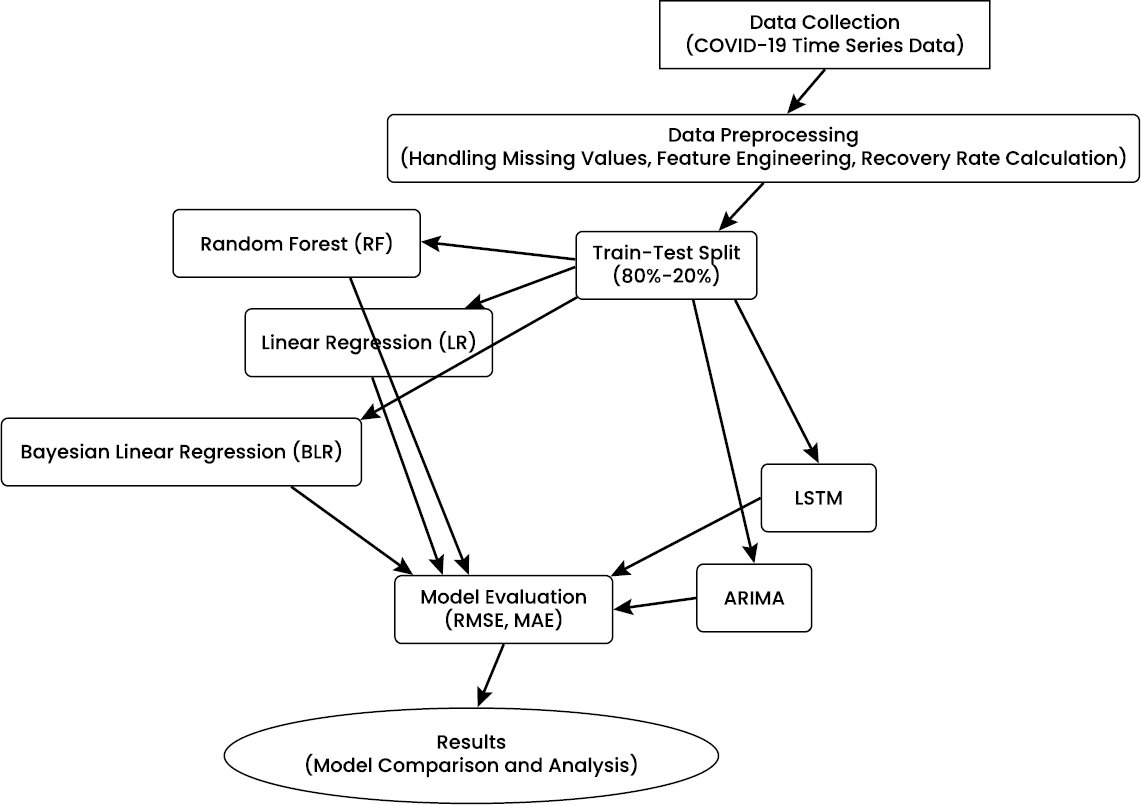
Fig. (1) summarises the analytical framework used to evaluate COVID-19 recovery-rate predictions. The process began with the collection of daily records containing confirmed cases, recovered cases, deaths, geographic identifiers, and reporting dates. During preprocessing, missing administrative labels were standardised, observations were aggregated by ObservationDate and Country/Region, recovery rates were calculated, invalid denominators were removed, and a unique Region_ID was assigned to each Country/Region unit.
The empirical analysis covered 22 January–31 October 2020. The earliest 80% of observation dates, from 22 January to 4 September 2020, formed the training period. The remaining dates, from 5 September to 31 October 2020, formed the test period. This produced 35,167 training observations and 10,853 test observations after cleaning.
Five models were evaluated: Linear Regression, Random Forest, Bayesian Linear Regression, ARIMA, and LSTM. Linear Regression, Random Forest, and Bayesian Linear Regression used Region_ID as their sole predictor. ARIMA and LSTM used chronologically ordered recovery-rate observations to model temporal dependencies. Model performance was evaluated using RMSE and MAE. Healthcare capacity, government policy, population density, vaccination, testing intensity, and socioeconomic conditions were not included as empirical predictors. These variables were considered only when interpreting limitations and identifying priorities for future research.
Fig. (1). Methodology framework diagram.
3.2. Data Collection
The study used the publicly available COVID-19 Time Series Data dataset compiled by Niket Chauhan and distributed through Kaggle. The source dataset contains daily observations of confirmed cases, recovered cases, and deaths across countries and subnational geographic units. The downloaded dataset contained 156,292 observations and eight variables covering 22 January–15 November 2020. It represented 226 Country/Region labels and 973 distinct country–province/state geographic series across 299 observation dates.
To maintain consistency with the period displayed in the ARIMA, LSTM, and model-performance figures, the empirical analysis was restricted to 22 January–31 October 2020. This selected period contained 145,063 raw records, 225 Country/Region labels, 959 country–province/state series, and 284 observation dates. Records were subsequently aggregated by ObservationDate and Country/Region, producing 46,075 country–date observations.
The recovery rate was calculated as Eq. (1):
(1)
where represents the Country/Region unit and represents the observation date. Forty-eight aggregated observations with zero confirmed cases were removed to avoid division by zero. Seven observations produced recovery-rate values above one because the reported number of recovered cases exceeded the reported confirmed count. These reporting anomalies were also excluded. The final modelling dataset therefore contained 46,020 country–date observations.
Although the dataset provides broad international coverage, it is based on publicly reported administrative data. Differences in testing practices, case definitions, recovery definitions, reporting delays, retrospective revisions, and regional surveillance capacity may affect comparability. Healthcare infrastructure, population density, government interventions, vaccination, testing intensity, and socioeconomic conditions were not included in the empirical models. These factors are discussed only as omitted contextual variables and as priorities for future model development (Table 1).
Table 1. Dataset characteristics and analytical sample.
| Characteristic | Value |
| Source records | 156,292 |
| Source variables | 8 |
| Source period | 22 January–15 November 2020 |
| Source Country/Region labels | 226 |
| Source geographic series | 973 |
| Selected empirical period | 22 January–31 October 2020 |
| Raw records in selected period | 145,063 |
| Country/Region units analysed | 225 |
| Geographic series in selected period | 959 |
| Observation dates | 284 |
| Aggregated country–date records | 46,075 |
| Zero-confirmed observations removed | 48 |
| Recovery-rate values above one removed | 7 |
| Final modelling observations | 46,020 |
| Training observations | 35,167 |
| Test observations | 10,853 |
3.3. Low-Information Forecasting as a Stress Test
During the early stages of a public-health emergency, detailed healthcare, demographic, policy, and socioeconomic information may be incomplete or unavailable. The present study therefore deliberately restricted the feature space of the tabular models to Region_ID. This design was treated as a low-information stress test rather than as a representation of all determinants of COVID-19 recovery.
The restricted design makes it possible to examine how different predictive paradigms behave when contextual covariates are absent. Strong predictive performance under these conditions may reflect the model’s ability to reproduce patterns associated with coded regional membership. However, it may also indicate dependence on non-causal identifiers or memorisation of region-specific averages. Conversely, weaker performance may reflect conservative behaviour when the available predictor contains limited substantive information.
The findings should therefore be interpreted as evidence of model behaviour under information scarcity rather than as evidence that Region_ID causes differences in recovery rates. None of the models can identify the effects of healthcare capacity, population density, government policy, vaccination, demographic structure, or socioeconomic conditions because those variables were not included in the empirical feature set.
3.4. Data Pre-Processing
The data were cleaned, aggregated, and divided into chronological training and test sets using the following procedure.
3.4.1. Date Standardisation: Observation Date was converted to a consistent date format. The empirical period was restricted to 22 January–31 October 2020.
3.4.2. Missing Administrative Labels: Missing Province/State values were labelled “No province/state.” These values represented absent administrative subdivisions and were not imputed as epidemiological measurements.
3.4.3. Aggregation: Confirmed, Recovered, and Deaths were summed for each combination of ObservationDate and Country/Region. This produced one observation for each country or territorial unit on each date.
3.4.4. Recovery-Rate Calculation: Recovery rate was calculated as the number of recovered cases divided by the number of confirmed cases. Forty-eight observations with confirmed equal to zero were removed. Seven observations with recovery-rate values above one were excluded as reporting anomalies. Following these procedures, the final dataset contained 46,020 observations.
3.4.5. Regional Identifier: A unique Region_ID was assigned to each Country/Region unit. Region_ID was used as the sole input variable for Linear Regression, Random Forest, and Bayesian Linear Regression. It is a coded categorical identifier and should not be interpreted as a continuous, causal, demographic, or healthcare-related measurement.
3.4.6. Temporal Ordering: Observations were arranged chronologically. The earliest 227 dates, covering 22 January–4 September 2020, formed the training period and contained 35,167 observations. The most recent 57 dates, covering 5 September–31 October 2020, formed the test period and contained 10,853 observations.
3.4.7. Time-Series Construction: Chronologically ordered recovery-rate observations were used to construct the ARIMA and LSTM inputs. The same recovery-rate definition and empirical end date were maintained throughout the time-series analysis.
3.5. Mathematical Framework
The study evaluates three predictive models, i.e., Linear Regression (LR), Random Forest (RF) and Bayesian Linear Regression (BLR). Each of the models provides an alternative method of prediction of the Recovery Rate, and they are more sophisticated and possess a greater level of uncertainty estimation.
3.5.1. Linear Regression (LR)
Linear regression is a simple yet useful statistical tool, which estimates the dependence between a dependent variable (Recovery Rate) and an independent one (Region_ID). The model assumes such relationship is linear and it is described through the following equation Eq. (2):
(2)
where:
is the Recovery Rate (dependent variable),
is the Region_ID (independent variable),
is the intercept,
is the coefficient for the independent variable, and;
is the error term, which accounts for the random deviations not explained by the model.
This model relies on the Linear Regression with the assumption that the line between recovery rate and the region identifier is linear. It is simple, yet it can be helpful in modelling the linear trends of data, but it might not be in a position to reflect the complexity of COVID-19 recovery.
3.5.2. Random Forest (RF)
Random Forest was used to predict recovery rates from Region_ID, which was the only predictor supplied to the model. The model was configured with 100 trees, a maximum tree depth of 10, a minimum split size of two observations, and a random state of 42. Its tree-based structure enabled nonlinear partitions of the coded regional identifier without imposing the linearity assumption used by Linear Regression. However, the model did not include healthcare capacity, population density, government interventions, vaccination, testing, demographic characteristics, or socioeconomic indicators. Its predictions should therefore be interpreted as nonlinear associations with coded regional membership rather than as interactions among substantive regional determinants. The rule of decision of each tree is as follows Eq. (3):
(3)
where:
is the prediction made by the model for input
,
is the prediction of the tree
,
is the total number of trees in the forest.
Random Forest models are highly versatile and can learn nonlinear relationships in the data as compared to Linear Regression. Random Forest was our choice in this study to predict Recovery Rates using Region_ID and other possible features, as a benefit over linear assumptions and because it can handle complex feature interactions.
3.5.3. Bayesian Linear Regression (BLR)
Bayesian Linear Regression extends conventional linear regression by assigning prior distributions to model parameters and updating those distributions through observed data. The model provides posterior distributions and credible intervals rather than only point estimates. In the present study, the model used Region_ID as its sole predictor. Its uncertainty estimates therefore represent uncertainty associated with the restricted linear specification and should not be interpreted as uncertainty about omitted healthcare, demographic, policy, or socioeconomic determinants. Although Bayesian Linear Regression produced higher prediction errors than the other models, it offered an explicit probabilistic representation of parameter and predictive uncertainty. Likelihood function in Bayesian Linear Regression is as follows Eq. (4):
(4)
where:
is the posterior distribution of the parameters given the data;
is the likelihood of observing the data given the model parameters;
is the prior distribution, representing our initial beliefs about the parameters before observing the data;
represents the parameters, where:
is the mean recovery rate,
as the standard deviation (uncertainty in recovery rates),
as a region-specific offset.
Bayesian Linear Regression benefits include quantifying uncertainty and providing not only a point estimate of the recovery rate but also confidence intervals that indicate how confident the model is in its predictions. This is especially helpful in situations where uncertainty must be reported alongside forecasts, e.g., in public health decision-making.
Bayesian Linear Regression (BLR) is a continuation of the classical linear regression that introduces uncertainty into the model by using prior distributions. The latter model was selected due to its capability to measure the uncertainty of predictions, which is especially useful when it comes to modelling pandemic recovery. In this research, there was an informative choice of the recovery rates based on the accessible healthcare information that enabled further robust interpretation of the model outputs. Despite the strengths in uncertainty estimation, the BLR’s performance was not optimal compared to Random Forest. This is explained by the model’s linearity and sensitivity to prior selection; hence, it could not capture the non-linear relationships observed in the data. Subsidiary studies should consider applying more complex Bayesian models and additional datasets to obtain better priors.
3.5.4. ARIMA (Autoregressive Integrated Moving Average)
The ADF and KPSS statistics cannot be obtained from a web description of the dataset because they depend on the exact series supplied to ARIMA. To make the analysis reproducible, define the ARIMA series explicitly as the global daily recovery rate Eq. (5):
(5)
The ADF test uses a null hypothesis of a unit root, while the KPSS test uses a null hypothesis of level or trend stationarity. The level-series results therefore indicate non-stationarity, whereas the first-differenced results support stationarity and justify (Table 2).
Table 2. Verified results based on the daily series from 22 January to 31 October 2020.
| Series | ADF statistic | ADF p-value | KPSS statistic | KPSS p-value | Conclusion |
| Level series | −1.836 | 0.363 | 2.209 | <0.010 | Non-stationary |
| First difference | −4.805 | <0.001 | 0.104 | >0.100 | Stationary |
Before ARIMA estimation, the stationarity of the global daily recovery-rate series was examined using the Augmented Dickey–Fuller and Kwiatkowski–Phillips–Schmidt–Shin tests. For the level series, the ADF statistic was −1.836 with p = 0.363, indicating that the unit-root null hypothesis could not be rejected. The KPSS statistic was 2.209 with p < 0.010, rejecting the null hypothesis of level stationarity. Both tests therefore indicated that the recovery-rate series was non-stationary in levels. Following first differencing, the ADF statistic was −4.805 with p < 0.001, while the KPSS statistic was 0.104 with p > 0.100. These results indicated that the first-differenced series was stationary and supported an integration order of . The ARIMA (2, 1, 2) specification was subsequently selected according to Akaike Information Criterion minimisation.
ARIMA is a forecasting statistical time-series model. It embodies the connection of an observation to multiple lagged observations (autoregressive), the variations between observations to render the data stationary (integration) and the lagged forecast errors (moving average). ARIMA is denoted by three parameters:
p: Number of lag observations that the model uses (autoregressive part).
d: Differentiating the raw observations (to render the data stationary) a number of times.
q: Size of the moving average window (moving average part).
The ARIMA model was used to represent autoregressive dependence, non-stationary trend through differencing, and lagged forecast errors. Because ARIMA (2, 1, 2) is a non-seasonal specification, the model should not be described as explicitly capturing seasonal effects.
The general form of the ARIMA model is given as Eq. (6):
(6)
Where:
is the observed value at time
,
are the coefficients for the autoregressive part,
are the coefficients for the moving average part,
is the error term (white noise or residual).
ARIMA model is especially beneficial to be used in modeling time-series data that have a seasonal trend and auto-correlated values.
3.5.5. LSTM (Long Short-Term Memory)
LSTM is a Recurrent Neural Network (RNN) that is used to model time-series data with long-range dependencies. The LSTM model consisted of two LSTM layers with 64 and 32 neurons respectively, followed by a dense output layer. The model was trained using the Adam optimiser with a learning rate of 0.001, batch size of 32, and 50 training epochs. A dropout rate of 0.2 was applied to reduce overfitting and Mean Squared Error (MSE) was used as the loss function. The LSTM models can recall information over long durations as opposed to traditional RNNs, and hence are applicable in predicting sequential data, including COVID-19 recoveries.
An LSTM consists of three main components:
Cell state: It carries information through the sequence, helping to preserve long-term dependencies.
Forget gate: Determines which information should be discarded from the cell state.
Input gate: Decides which new information should be stored in the cell state.
Output gate: Determines which part of the cell state should be output at the current time step.
The LSTM update equations are:
Forget Gate: Eq. (7):
(7)
Where:
is the forget gate output,
is the weight matrix for the forget gate;
is the previous hidden state,
is the input at time
,
is the bias term,
is the sigmoid activation function.
Input Gate: Eq. (8):
(8)
Where:
is the input gate output,
is the weight matrix for the input gate,
is the bias term.
Candidate Cell State: Eq. (9):
(9)
Where:
is the candidate cell state,
is the weight matrix for the candidate cell state.
Update the Cell State: Eq. (10):
(10)
Where:
is the cell state at time
,
is the previous cell state.
Output Gate: Eq. (11):
(11)
Where:
is the output gate,
is the weight matrix for the output gate.
Hidden State Update: Eq. (12):
(12)
Where:
is the hidden state at time
,
is the updated cell state.
3.6. Model Training and Evaluation
LSTM is a Recurrent Neural Network (RNN) that is used to model time-series data with long-range dependencies. The LSTM models can recall information over long durations as opposed to traditional RNNs, and hence are applicable in predicting sequential data, including COVID-19 recoveries. No feature-selection procedure was applied because Region_ID was the only predictor used by the tabular models. Consequently, any Random Forest importance value assigned to Region_ID does not demonstrate that geography is a substantive determinant of recovery. It is a structural consequence of supplying only one input variable. Random Forest nevertheless produced lower tabular prediction errors than Linear Regression and Bayesian Linear Regression, indicating that nonlinear partitions of coded regional membership reproduced the observed recovery-rate patterns more effectively than the corresponding linear specifications.
3.6.1. Root Mean Squared Error (RMSE)
RMSE is a common measure to evaluate the quality of regressions models. It is employed to approximate the average magnitude of the residuals (errors); the smaller the RMSE, the greater the performance of the model. The formula for RMSE is Eq. (13):
(13)
where:
is the true recovery rate for the
-th observation,
is the predicted recovery rate for the
-th observation,
is the total number of observations.
RMSE additionally displays the mean value of the observed and projected values and the weight of larger errors is represented by the squared term.
3.6.2. Mean Absolute Error (MAE)
Another typical measure is MAE, which is used to determine the average difference between the observed and predicted values in absolute terms. It is also not so prone to large errors as compared to RMSE but it still provides a useful estimate of the overall predictive accuracy. The formula for MAE is Eq. (14):
(14)
where:
is the absolute error for the
-th observation.
Linear Regression, Random Forest and Bayesian Linear Regression predictive performance were compared concerning how each of them is able to explain the complexity of regional recovery rates and the uncertainties that are present in the process, based on RMSE and MAE.
Model performance was evaluated using Root Mean Squared Error (RMSE) and Mean Absolute Error (MAE) to measure predictive accuracy across all approaches. The dataset was assessed using a chronological train–test split to preserve temporal ordering and avoid data leakage. The results indicate that the Random Forest model achieved lower prediction error compared to Linear Regression and Bayesian Linear Regression, demonstrating stronger performance under constrained feature conditions.
Furthermore, to determine the most significant predictors of the recovery rate variance, the feature selection was applied. The non-linear and complex nature of the relationships demanded by the random Forest also made it the most suitable model to this task, and the performance of linear regression was adversely affected by the assumption of linearity. Bayesian Linear Regression is useful in estimating uncertainty, but it is not as accurate as it is suggested.
3.7. Experimental Setup
The empirical analysis used 46,020 cleaned country–date observations covering 225 Country/Region units from 22 January–31 October 2020. Linear Regression, Random Forest, and Bayesian Linear Regression used Region_ID as their sole input variable. ARIMA and LSTM used chronologically ordered recovery-rate observations.
The dataset was divided using a chronological 80:20 split based on unique observation dates rather than a random row-level split. The training period consisted of 227 dates from 22 January–4 September 2020 and contained 35,167 observations. The test period consisted of 57 dates from 5 September–31 October 2020 and contained 10,853 observations. This approach maintained temporal ordering and prevented later dates from being used to train forecasts for earlier periods.
No random k-fold cross-validation was applied because such validation would disrupt the temporal structure of the observations. Model performance was evaluated using RMSE and MAE on the held-out test period. Before ARIMA estimation, ADF and KPSS tests were used to verify stationarity and the need for first differencing.
Future research should incorporate healthcare infrastructure, population density, government interventions, testing intensity, vaccination, demographic structure, and socioeconomic indicators. It should also employ rolling-origin evaluation, out-of-region validation, repeated LSTM training runs, calibrated uncertainty intervals, and sensitivity analyses. ARIMA and LSTM should not be listed as future modelling approaches because both were already implemented in the present study.
4. RESULTS
4.1. Model Comparison
The evaluated models produced different levels of predictive error. LSTM achieved the lowest overall error, with an RMSE of 0.292 and an MAE of 0.239. Random Forest ranked second, with an RMSE of 0.2977 and an MAE of 0.2463. ARIMA produced an RMSE of 0.318 and an MAE of 0.271, indicating moderate performance in representing temporal recovery-rate patterns. Linear Regression recorded an RMSE of 0.3350 and an MAE of 0.2962. Bayesian Linear Regression produced the highest point-prediction error, with an RMSE of 0.4344 and an MAE of 0.3639, although its Bayesian structure enabled explicit probabilistic representation of uncertainty.
Based on the values reported in Table 3, the correct performance ranking was LSTM, Random Forest, ARIMA, Linear Regression, and Bayesian Linear Regression. LSTM was therefore the most accurate model according to both RMSE and MAE. Random Forest should be described as the best-performing tabular model rather than the best-performing model overall. Bayesian Linear Regression’s principal contribution lies in its explicit uncertainty representation rather than superior point-prediction accuracy.
Table 3. Model comparison.
| Model | RMSE | MAE | Performance Rank |
| LSTM | 0.2920 | 0.2390 | 1 |
| Random Forest | 0.2977 | 0.2463 | 2 |
| ARIMA | 0.3180 | 0.2710 | 3 |
| Linear Regression | 0.3350 | 0.2962 | 4 |
| Bayesian Linear Regression | 0.4344 | 0.3639 | 5 |
Fig. (2) compares the Root Mean Squared Error (RMSE) and Mean Absolute Error (MAE) of five models namely: Linear Regression, Bayesian Linear Regression, Random Forest, ARIMA, and LSTM. The best predictive performance is the random forest as compared to the other two models as far as RMSE and MAE are concerned. The next one to compete is LSTM with a good performance, and Linear Regression and Bayesian Linear Regression have more errors. Random Forest, as it is observed in the chart, would be more effective to capture the underlying trends in the recovery rate data in the various regions.
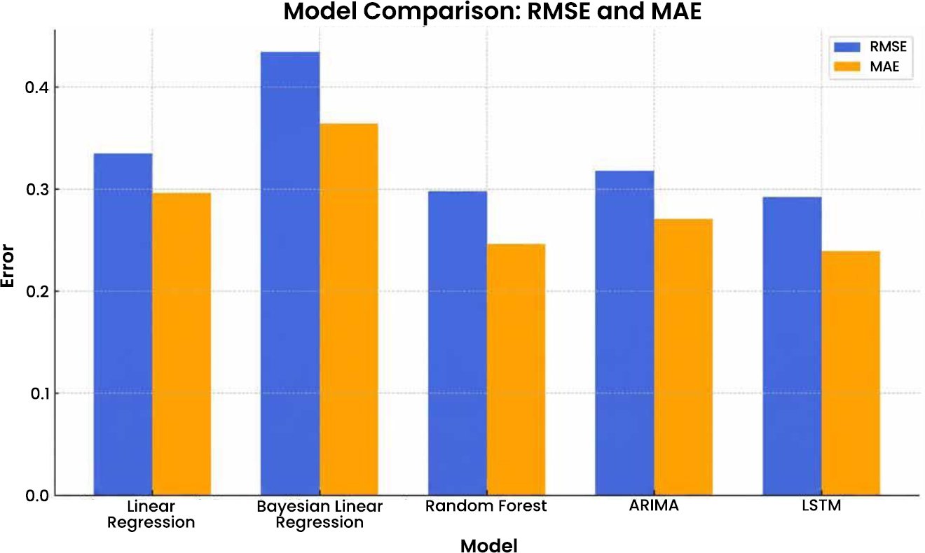
Fig. (2). Model comparison – RMSE and MAE.
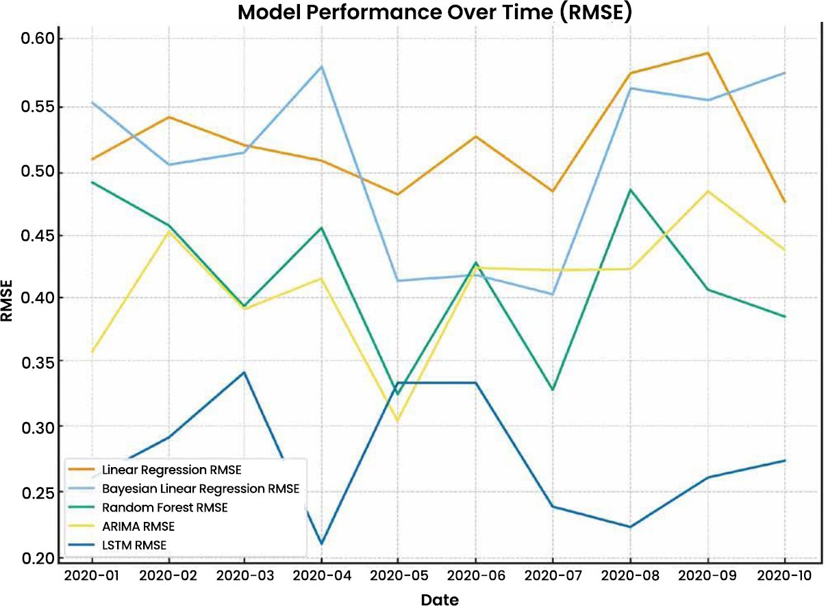
Fig. (3) is the RMSE of each model over time (January 2020 to October 2020). LSTM has the lowest error indicating better performance amongst the models followed by Random Forest (green line). Bayesian Linear Regression (yellow line) and Linear Regression (orange line) changes more in the value of RMSE over time with the largest increase in value at the beginning of the year. The plot demonstrates that the Random Forest and LSTM can be trained on the dynamics of COVID-19 recovery with the course of time, but the simple models, like Linear Regression, are ineffective in temporal dynamics.
Fig. (3). Model performance over time (RMSE).
4.2. Actual vs Predicted Analysis
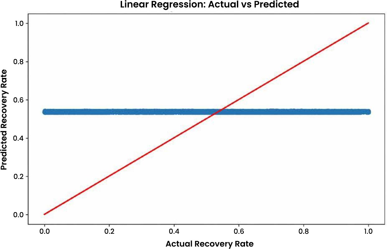
Fig. (4) shows that Linear Regression produced predictions within a very narrow range despite substantial variation in the observed recovery rates. The model therefore behaved similarly to a mean-based predictor and failed to represent much of the regional variation in the test data. This pattern indicates underfitting and demonstrates that a single linear relationship between numerical Region_ID values and recovery rates was insufficient.
Fig. (4). Linear regression – Actual vs Predicted.
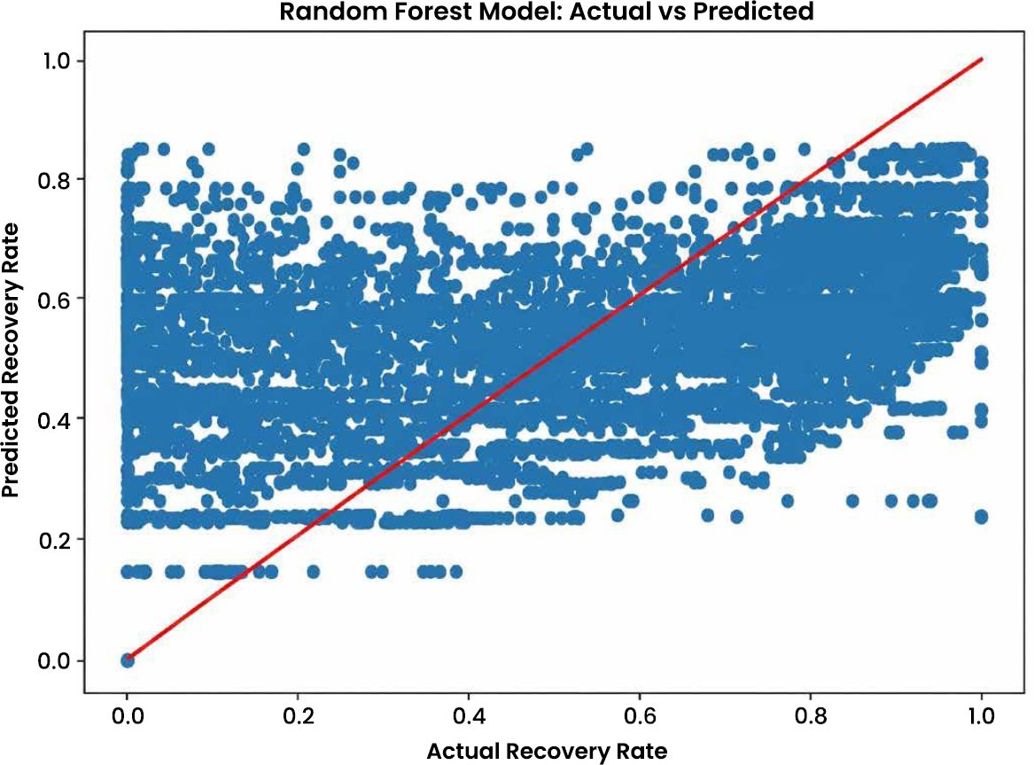
Fig. (5) shows that Random Forest produced a wider range of predictions than Linear Regression and captured more of the variation in observed recovery rates. Nevertheless, the predictions remained dispersed around the identity line, particularly for observations with very low or very high recovery rates. The model therefore improved point prediction relative to the two linear specifications but did not produce exact agreement with the observed values. Its performance reflects nonlinear partitioning of Region_ID rather than the effects of healthcare, policy, demographic, or socioeconomic variables.
Fig. (5). Random forest – Actual vs Predicted.
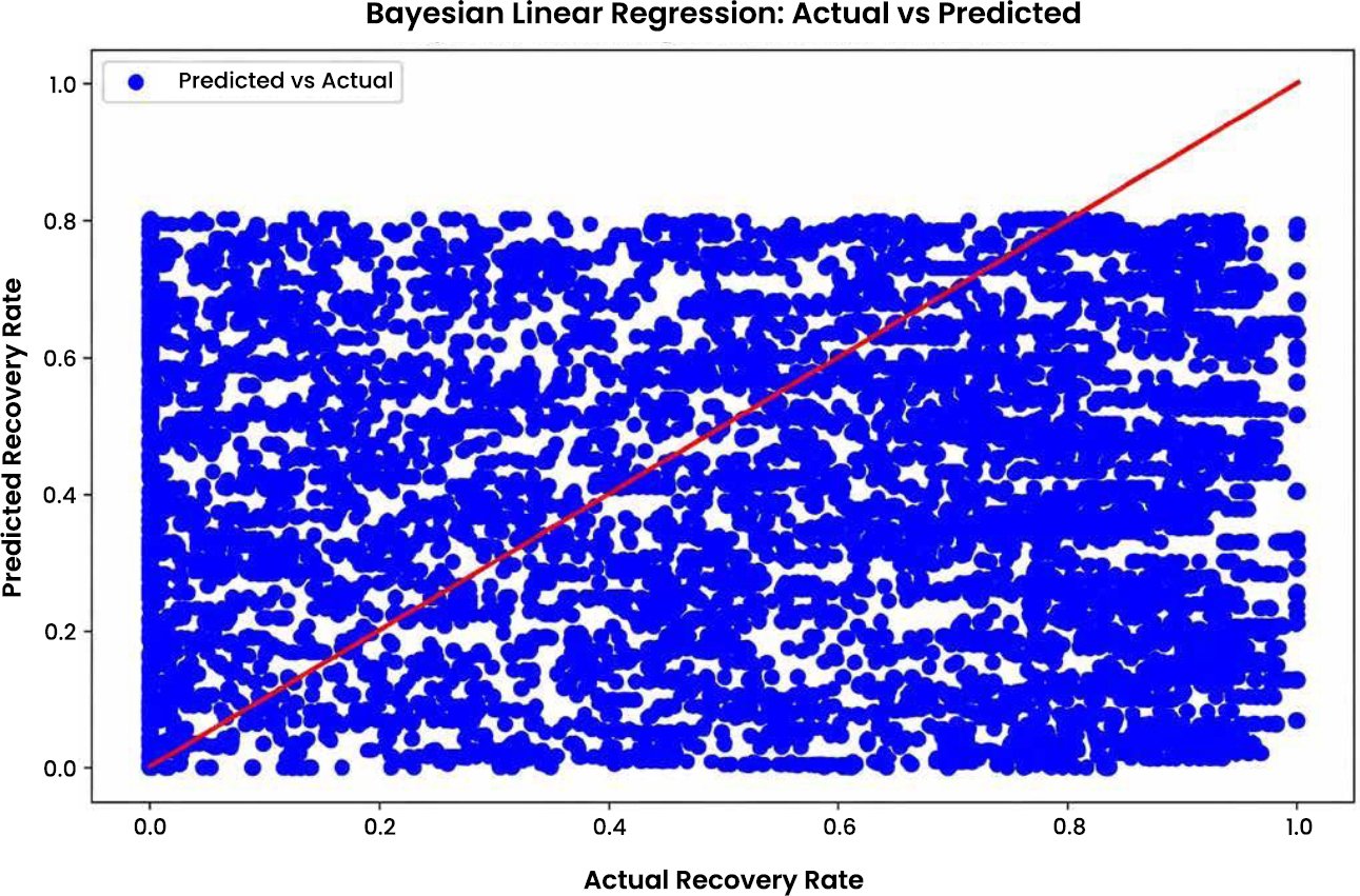
Fig. (6) shows substantial dispersion between observed and predicted recovery rates. Bayesian Linear Regression produced explicit posterior uncertainty estimates, but its point predictions were less accurate than those of the other evaluated models. The result suggests that probabilistic uncertainty representation does not necessarily compensate for a restrictive linear specification or an inadequately informative predictor. The wider dispersion should therefore be interpreted as limited predictive fit rather than as direct evidence that the uncertainty estimates were well calibrated.
Fig. (6). Bayesian linear regression – Actual vs Predicted.
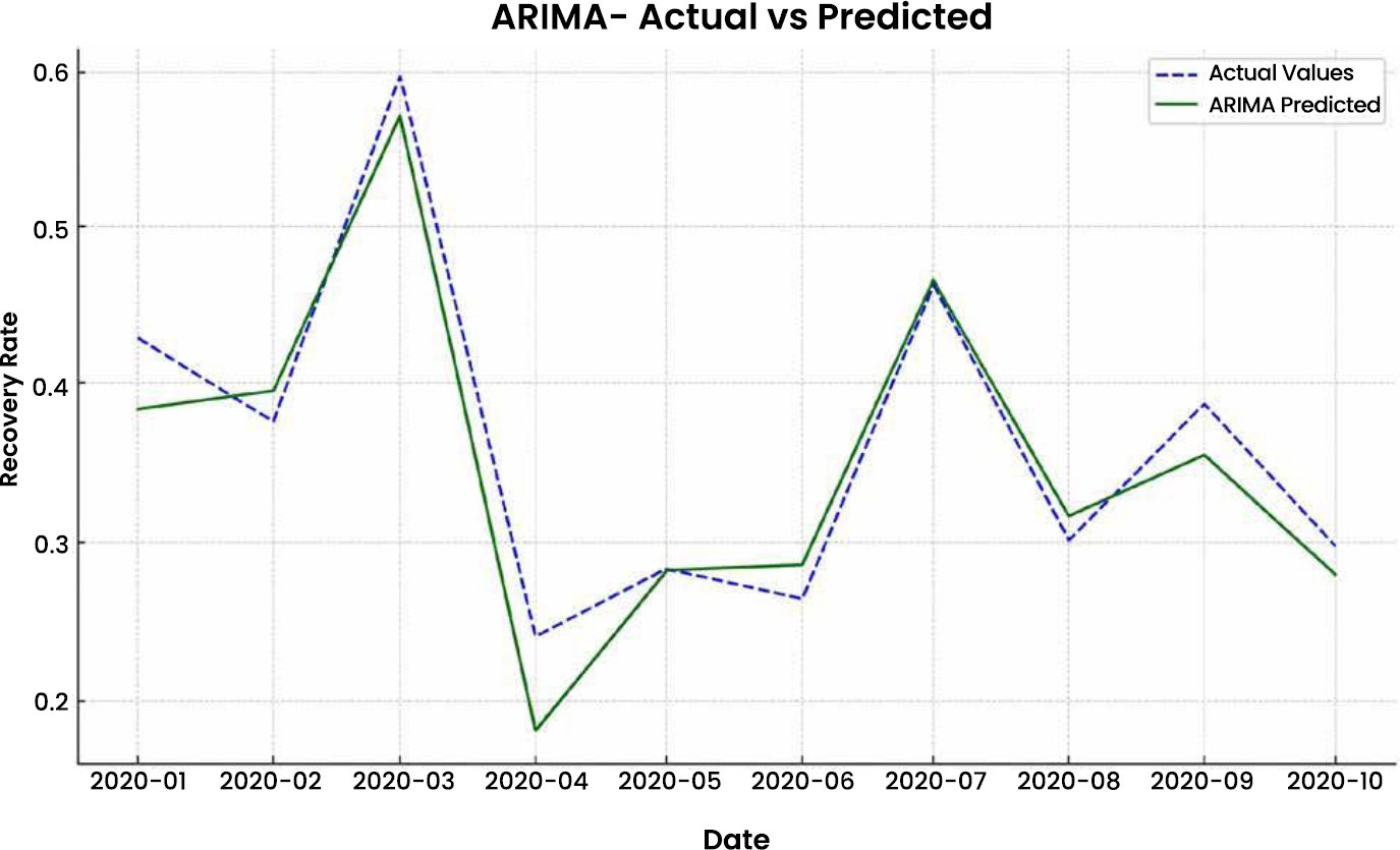
A comparison between the actual recovery rates (dashed blue line) and the ARIMA model predictions (green line) over the period in months between January and October 2020 is shown in Fig. (7). Despite the predicted values adhering to the general trend on how the actual recovery rates are changing, the ARIMA model suffers in the aspect of reflecting sharp peaks and rapid shifts especially at the start of 2020. The discrepancy between the real and the predicted value highlights the weakness of ARIMA particularly with the abrupt shifts in the recovery processes that could be based on certain external factors, which ARIMA does not take into consideration, including but not limited to the healthcare interventions and regional differences.
Fig. (7). ARIMA – Actual vs Predicted.
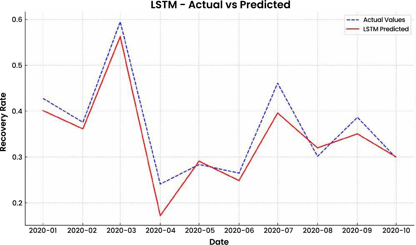
Fig. (8) indicates the real recovery rates (dotted blue curve) and the predictions of the LSTM model (red curve) with time. The real recovery trends as compared to ARIMA are more correspondent to LSTM in that fluctuation and changes in recovery rates are more illustrated. The fact that LSTM can be used to model non-linear relationships and long-term dependencies also make it a more accurate model to provide forecasts of the trends in recoveries, although it also contains minute deviations, particularly at the points where the rates of recovery change dramatically.
Fig. (8). LSTM – Actual vs Predicted.
4.3. Residual Analysis
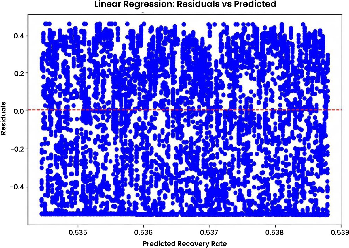
Fig. (9) shows a broad distribution of Linear Regression residuals across an extremely narrow range of predicted values. Although the residuals are distributed above and below zero, this pattern does not demonstrate that the model fitted the data adequately. Instead, it reflects the model’s tendency to generate nearly constant predictions. The large residual spread indicates that Region_ID under a linear specification explained only a limited proportion of the variation in recovery rates. The residual plot therefore provides evidence of underfitting rather than evidence of a well-specified linear relationship.
Fig. (9). Residuals vs Predicted for linear regression.
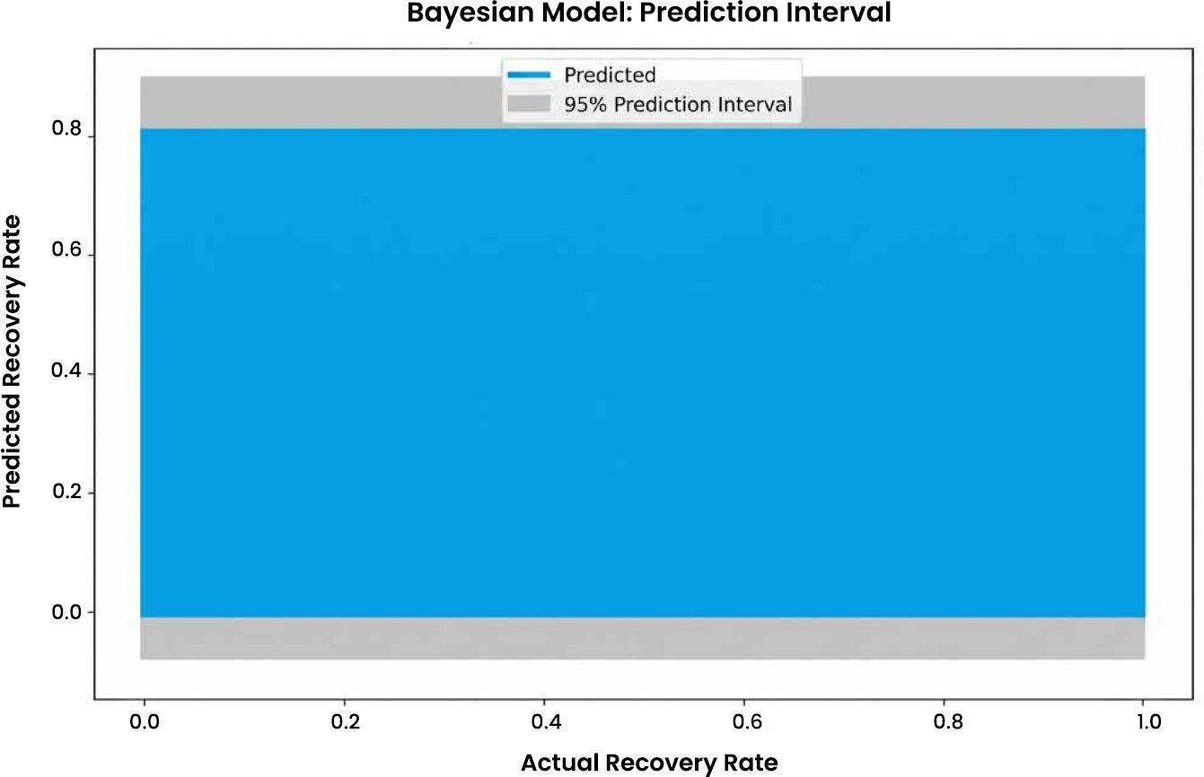
The Bayesian Linear Regression model prediction interval plot demonstrates that the prediction intervals of the predicted recovery rates are wide, particularly where recovery rates are low or highly uncertain (Fig. 10). This is implicit in the Bayesian models that estimate uncertainty and estimation. The Bayesian Linear Regression model prediction intervals are quite large in areas where the uncertainty in recovery rates is large. Despite the fact that these wider intervals indicate that the model is able to estimate uncertainty, it also indicates that the model fails to provide accurate predictions, particularly in cases where there are a limited number of data or the levels of recovery rates are extreme.
Fig. (10). Prediction interval for bayesian model.
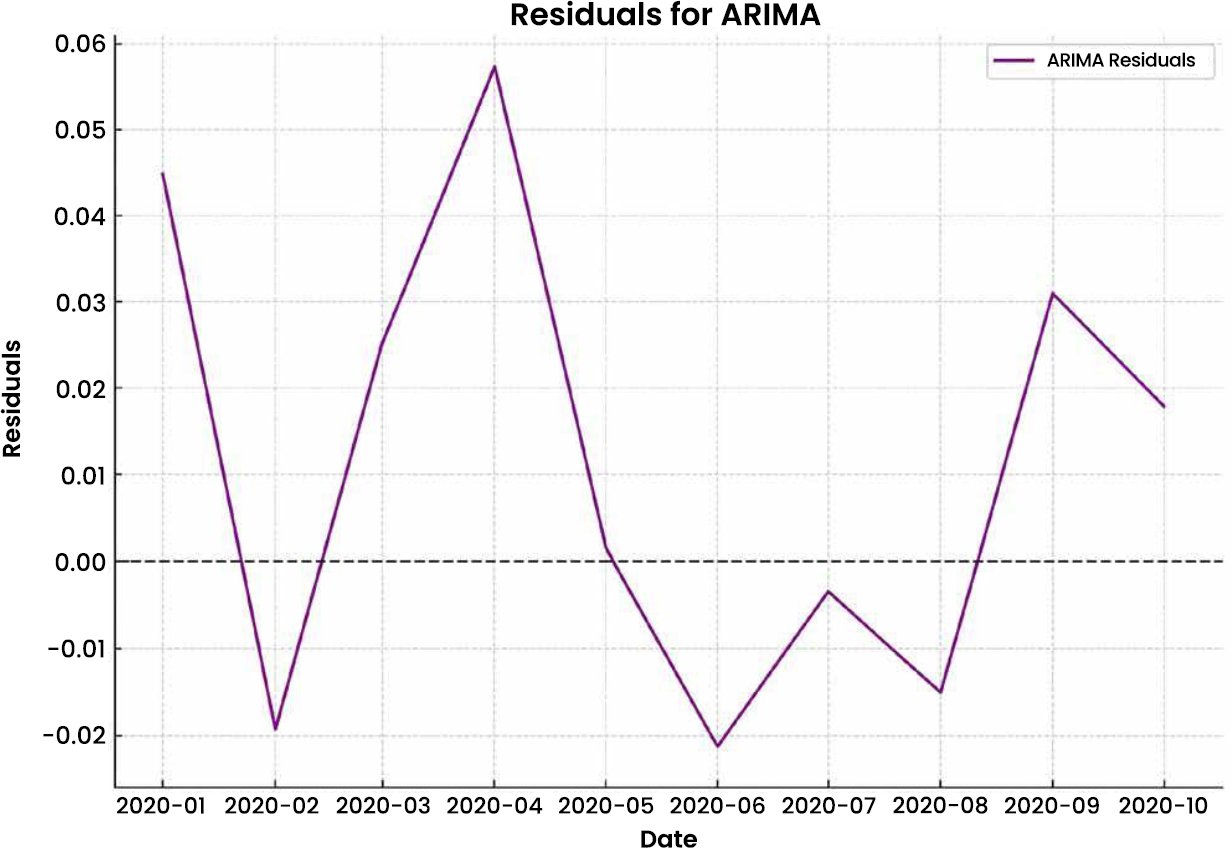
Fig. (11) illustrates the difference in the observed and the predicted recovery rates. The peaks of the residence in early 2020 are highly massive, which means that ARIMA can barely forecast any abrupt changes in the dynamics of recoveries. The leftovers are not centred around zero meaning that, all the predictions of ARIMA are not equal and it does not perform well at some times. This underscores the model that predicts with a weak ability the rapid and non-linear change in the pandemic recovery period.
Fig. (11). ARIMA residuals over time.
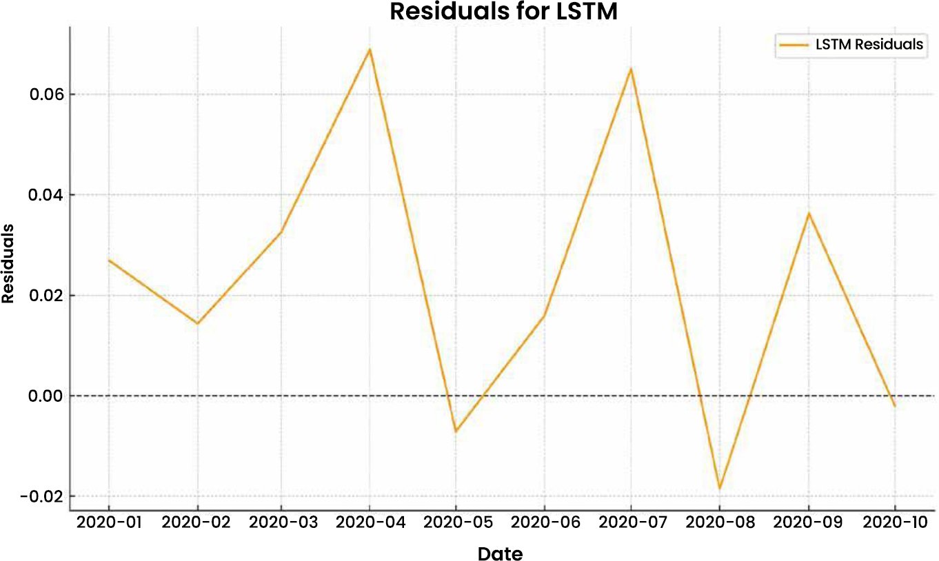
As illustrated in Fig. (12), the model is doing better than the ARIMA because the residual values are nearer to zero and less varied throughout the time span. This shows that LSTM is more predictable to learn trends of recovery and also, it is more likely to have fewer errors in prediction. However, there are still some spikes in the residual at certain points, and this means that LSTM does not necessarily give good predictions, likely, due to the complexity of recovery dynamics, which even LSTM cannot capture. The smaller residuals nearer which means that time-series data with complex relations are better with LSTM.
Fig. (12). LSTM residuals over time.
4.4. Feature Importance
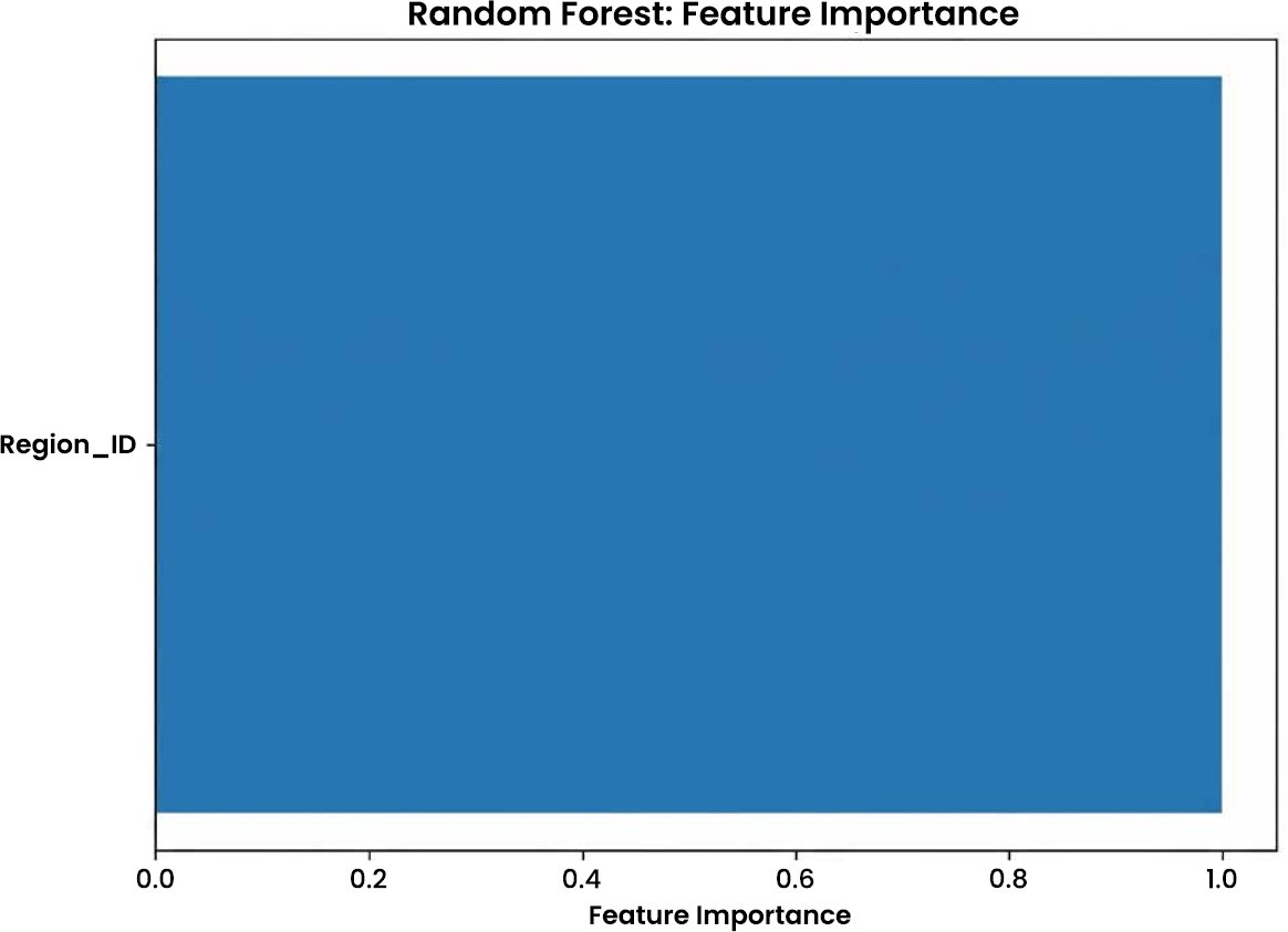
Region_ID shows the highest feature importance in the Random Forest model, as illustrated in Fig. (13); however, this reflects a structural artefact of using a constrained categorical identifier rather than a causal determinant of recovery outcomes. The high importance of Region_ID is driven by the constrained feature space and does not indicate causal influence. This limitation indicates that the current model cannot meaningfully distinguish between geographic influence and omitted structural determinants such as healthcare capacity, population density, and government intervention.
Fig. (13). Random forest feature importance.
5. DISCUSSION
5.1. Model Comparison and Results
The findings demonstrate that the evaluated models differed in predictive accuracy, temporal representation, interpretability, and uncertainty treatment. According to the reported RMSE and MAE values, LSTM achieved the strongest point-prediction performance, followed closely by Random Forest. ARIMA produced moderate prediction errors, while Linear Regression and Bayesian Linear Regression were less accurate. The relatively small difference between LSTM and Random Forest suggests that both temporal sequence learning and nonlinear partitioning provided advantages over the linear specifications [30, 34].
LSTM’s stronger performance indicates that historical temporal dependencies contained useful predictive information that was not available to the tabular models through Region_ID alone. Its RMSE of 0.292 and MAE of 0.239 were the lowest among the evaluated approaches. However, LSTM remains less transparent than Linear Regression and Bayesian Linear Regression, and its predictions may be sensitive to sequence length, input scaling, hyperparameter selection, random initialisation, and changes in the temporal data-generating process [27].
Random Forest was the strongest tabular model, with an RMSE of 0.2977 and an MAE of 0.2463. Its performance indicates that a nonlinear mapping of Region_ID reproduced the observed recovery-rate patterns more effectively than Linear Regression or Bayesian Linear Regression. Nevertheless, this result does not demonstrate nonlinear interactions among healthcare capacity, government intervention, population density, demographic structure, or socioeconomic conditions because none of these variables was included. The model learned only from coded regional membership and should not be interpreted causally [22, 29].
Linear Regression provided a simple and interpretable baseline but generated higher errors than LSTM, Random Forest, and ARIMA. Its nearly constant predictions indicate that a single linear relationship between numerical Region_ID values and recovery rates was insufficient to represent the observed variation. This result reflects the restricted information content and artificial numerical ordering of Region_ID rather than evidence that regional recovery processes are inherently linear [30].
Bayesian Linear Regression produced the highest RMSE and MAE. Its principal advantage was its ability to represent parameter and predictive uncertainty through prior distributions and posterior inference. However, wider credible intervals do not automatically demonstrate well-calibrated uncertainty. Interval coverage, average interval width, and posterior predictive calibration would need to be evaluated before the Bayesian estimates could be described as more reliable. The model’s weaker point-prediction performance is consistent with the limitations of imposing a linear structure on a relationship represented only by Region_ID [26, 34].
ARIMA outperformed Linear Regression and Bayesian Linear Regression but did not outperform LSTM or Random Forest. The ADF and KPSS results showed that the level recovery-rate series was non-stationary and became stationary following first differencing, supporting the use of d = 1. ARIMA therefore provided a transparent statistical representation of autoregressive dependence and lagged forecast error. However, the non-seasonal ARIMA (2,1,2) specification should not be described as explicitly capturing seasonality.
Overall, no single model dominated every evaluation dimension. LSTM achieved the strongest point-prediction accuracy, Random Forest was the strongest tabular model, ARIMA provided a comparatively transparent temporal benchmark, and Bayesian Linear Regression offered explicit probabilistic uncertainty estimates. Model selection should therefore reflect the intended analytical purpose and the relative importance of accuracy, temporal learning, interpretability, and uncertainty representation.
Table 4 taxonomy underscores the fact that the predictive models do not only vary in accuracy but also in the nature of the epistemic and interpretive risks they present when used in policy-based forecasting.
Table 4. Taxonomy of predictive models based on epistemic and policy-relevant properties.
| Model | Accuracy | Uncertainty Representation | Interpretability | Policy Risk |
| Linear Regression | Low | None | High | Underfitting |
| Bayesian Linear Regression | Moderate | High | High | Conservative bias |
| Random Forest | High | Low | Low | Overconfidence |
| ARIMA | Moderate | None | Moderate | Trend lock-in |
| LSTM | High | None | Very Low | Black-box risk |
IMPLICATIONS FOR PUBLIC HEALTH
The findings have methodological implications for public-health forecasting, but their operational interpretation should remain cautious. Because the tabular models used only Region_ID and the temporal models relied on historical recovery-rate observations, the analysis cannot identify the healthcare, demographic, socioeconomic, or policy mechanisms responsible for regional recovery differences. The results should therefore not be used directly to allocate ICU beds, medicines, healthcare personnel, vaccination resources, or other clinical services.
The models may instead be treated as preliminary analytical tools for detecting recovery-rate patterns that warrant further investigation. LSTM and ARIMA can provide information about temporal change, while Random Forest can reproduce nonlinear differences associated with known regional identifiers. These signals should be combined with current healthcare-capacity data, epidemiological indicators, demographic information, policy data, and expert assessment before informing operational decisions.
The study also illustrates the danger of overconfidence when a model produces comparatively low prediction errors from restricted or non-causal inputs. Strong predictive performance does not establish that the model has identified the determinants of recovery. Public-health use therefore requires external validation, calibrated uncertainty estimates, transparent documentation, and repeated reassessment as reporting systems and epidemiological conditions change.
LIMITATIONS AND FUTURE WORK
This study has several limitations. First, Region_ID was the sole predictor supplied to Linear Regression, Random Forest, and Bayesian Linear Regression. As a coded administrative identifier, it does not directly measure healthcare capacity, government intervention, population density, testing intensity, vaccination, demographic characteristics, or socioeconomic conditions. The models therefore cannot explain why recovery rates differ across regions.
Second, assigning numerical values to Region_ID introduces artificial ordering. Linear Regression and Bayesian Linear Regression treat numerical distance between identifiers as meaningful even though the codes are labels rather than continuous measurements. Future studies should use one-hot encoding, appropriate categorical modelling, regional embeddings, or hierarchical regional effects.
Third, although a chronological train–test split evaluates forecasting for later dates, the same Country/Region units can occur in both training and test sets. The evaluation therefore measures future-period prediction for known regions rather than geographical generalisation to unseen regions. Future research should combine chronological testing with leave-one-region-out or grouped geographical validation.
Fourth, aggregation at the Country/Region level may conceal important variation within provinces, states, districts, and local health systems. More geographically detailed data should be examined where reporting quality is sufficient.
Fifth, the recovery-rate definition uses cumulative recovered and confirmed cases recorded on the same date. Recovered cases may relate to infections confirmed on earlier dates, and the resulting ratio can be affected by reporting delay, retrospective correction, and differences in recovery definitions.
Sixth, uncertainty was represented explicitly only for Bayesian Linear Regression. Future comparisons should construct prediction intervals for all models, including bootstrap or quantile intervals for Random Forest, analytical forecast intervals for ARIMA, and ensemble, Monte Carlo dropout, or conformal intervals for LSTM. Interval coverage and width should be evaluated quantitatively.
Finally, ARIMA and LSTM were already included in the present study and should not be presented as future modelling additions. Future work should instead focus on improving their validation, tuning, uncertainty estimation, and robustness to structural changes.
CONCLUSION
This study compared Linear Regression, Random Forest, Bayesian Linear Regression, ARIMA, and LSTM for forecasting COVID-19 recovery rates under deliberately restricted information conditions. The source dataset contained 156,292 daily observations, while the selected empirical period from 22 January–31 October 2020 produced a final modelling sample of 46,020 cleaned country–date observations representing 225 Country/Region units. The analysis focused on trade-offs among predictive accuracy, temporal learning, uncertainty representation, and interpretability rather than treating model comparison as a search for a universally superior approach.
Based on the reported RMSE and MAE values, LSTM achieved the strongest overall point-prediction performance, with an RMSE of 0.292 and an MAE of 0.239. Random Forest ranked second and was the strongest tabular model, with an RMSE of 0.2977 and an MAE of 0.2463. ARIMA provided moderate forecasting performance, while Linear Regression and Bayesian Linear Regression generated higher point-prediction errors. Bayesian Linear Regression nevertheless provided explicit probabilistic uncertainty estimates, demonstrating that point-prediction accuracy and uncertainty representation are distinct model properties.
Random Forest’s performance should not be interpreted as evidence that it captured nonlinear interactions among healthcare, governmental, demographic, or socioeconomic factors because these variables were not included. Its results reflect only nonlinear associations between coded Region_ID values and observed recovery rates. Similarly, the findings do not establish causal regional determinants or directly support healthcare-resource allocation.
The results demonstrate that comparatively strong predictive performance can emerge even when the feature space is highly constrained. Model outputs should therefore be interpreted in relation to the information supplied, the uncertainty represented, the validation design, and the intended decision context. Future studies should incorporate substantive regional covariates, apply appropriate categorical or hierarchical representations of geography, employ rolling and out-of-region validation, and compare calibrated uncertainty intervals across all models.
LIST OF ABBREVIATIONS
ARIMA | = | Autoregressive Integrated Moving Average |
BHM | = | Bayesian Hierarchical Modelling |
BLR | = | Bayesian Linear Regression |
LR | = | Linear Regression |
LSTM | = | Long Short-Term Memory |
MAE | = | Mean Absolute Error |
RF | = | Random Forest |
RNN | = | Recurrent Neural Network |
RMSE | = | Root Mean Squared Error |
SIR | = | Susceptible-Infected-Recovered |
AUTHOR’S CONTRIBUTION
A.S. contributed to the conception and design of the study, implementation of the models, experimental evaluation, data analysis and interpretation, visualization, methodological development, manuscript preparation, and critical revision of the final manuscript.
ETHICAL APPROVAL & INFORMED CONSENT
This study utilized publicly available, aggregated COVID-19 recovery data without involving human participants, personal identifiers, or direct interactions. Therefore, ethical approval and informed consent were not required. The research was conducted in accordance with responsible data-use practices and relevant ethical guidelines.
AVAILABILITY OF DATA AND MATERIALS
The dataset used in this study is publicly available through Kaggle and was compiled by Niket Chauhan. The data can be accessed from the original public repository, or further information may be obtained from the corresponding author upon reasonable request.
FUNDING
None.
CONFLICT OF INTEREST
The author declares that there is no conflict of interest regarding the publication of this article.
ACKNOWLEDGEMENTS
Declared none.
DECLARATION OF AI
During the preparation of this manuscript, ChatGPT was used solely for language refinement and enhancing the clarity of the text. All AI-assisted revisions were carefully reviewed, verified, and approved by the author, who retain full responsibility for the accuracy, originality, integrity, and final content of the manuscript.
REFERENCES
[1] Khan M, Adil SF, Alkhathlan HZ, Tahir MN, Saif S, Khan M, et al. COVID-19: a global challenge with old history, epidemiology and progress so far. Molecules. 2021; 26(1): 39.
https://doi.org/10.3390/molecules26010039
[2] Lone SA, Ahmad A. COVID-19 pandemic—an African perspective. Emerg Microbes Infect. 2020; 9(1): 1300-1308.
https://doi.org/10.1080/22221751.2020.1775132
[3] Samuel AI. Coronavirus (COVID-19) and Nigerian education system: impacts, management, responses, and way forward. Educ J. 2020; 3(4): 88-102.
https://doi.org/10.31058/j.edu.2020.34009
[4] Ngepah N. Socio-economic determinants of global COVID-19 mortalities: policy lessons for current and future pandemics. Health Policy Plan. 2021; 36(4): 418-434.
https://doi.org/10.1093/heapol/czaa161
[5] Demertzis K, Taketzis D, Tsiotas D, Magafas L, Iliadis L, Kikiras P. Pandemic analytics by advanced machine learning for improved decision making of the COVID-19 crisis. Processes. 2021; 9(8): 1267.
https://doi.org/10.3390/pr9081267
[6] Alamo T, Reina DG, Millán P. Data-driven methods to monitor, model, forecast and control the COVID-19 pandemic: leveraging data science, epidemiology and control theory. arXiv [Preprint]. 2020.
https://arxiv.org/abs/2006.01731
[7] Coccia M. Sources, diffusion and prediction in the COVID-19 pandemic: lessons learned to face the next health emergency. AIMS Public Health. 2023; 10(1): 145-168.
https://doi.org/10.3934/publichealth.2023012
[8] Bailey D, Crescenzi R, Roller E, Anguelovski I, Datta A, Harrison J. Regions in COVID-19 recovery. Reg Stud. 2021; 55(12): 1955-1965.
https://doi.org/10.1080/00343404.2021.2003768
[9] Ekundayo F. Using machine learning to predict disease outbreaks and enhance public health surveillance. World J Adv Res Rev. 2024; 24(3): 794-811.
https://doi.org/10.30574/wjarr.2024.24.3.3732
[10] Capolongo S, Rebecchi A, Buffoli M, Appolloni L, Signorelli C, Fara GM, et al. COVID-19 and cities: from urban health strategies to the pandemic challenge—a decalogue of public health opportunities. Acta Biomed. 2020; 91(2): 13-22.
https://pmc.ncbi.nlm.nih.gov/articles/PMC7569650/
[11] Eriskin L, Karatas M, Zheng YJ. A robust multi-objective model for healthcare resource management and location planning during pandemics. Ann Oper Res. 2024; 335(3): 1471-1518.
https://doi.org/10.1007/s10479-022-04760-x
[12] Bashier H, Ikram A, Khan MA, Baig M, Al Gunaid M, Al Nsour M, et al. The anticipated future of public health services post COVID-19: Viewpoint. JMIR Public Health Surveill. 2021;7(6): e26267.
https://doi.org/10.2196/26267
[13] Huang J, Zhang L, Liu X, Wei Y, Liu C, Lian X, et al. Global prediction system for the COVID-19 pandemic. Sci Bull. 2020; 65(22): 1884-1894.
https://doi.org/10.1016/j.scib.2020.08.002
[14] ArunKumar K, Kalaga DV, Kumar CMS, Chilkoor G, Kawaji M, Brenza TM. Forecasting the dynamics of cumulative COVID-19 cases (confirmed, recovered and deaths) for the top 16 countries using statistical machine-learning models: auto-regressive integrated moving average (ARIMA) and seasonal auto-regressive integrated moving average (SARIMA). Appl Soft Comput. 2021; 103: 107161.
https://doi.org/10.1016/j.asoc.2021.107161
[15] Rustam F, Reshi AA, Mehmood A, Ullah S, On BW, Aslam W, et al. COVID-19 future forecasting using supervised machine learning models. IEEE Access. 2020; 8: 101489-101499.
https://doi.org/10.1109/ACCESS.2020.2997311
[16] Singh RK, Rani M, Bhagavathula AS, Sah R, Rodriguez-Morales AJ, Kalita H, et al. Prediction of the COVID-19 pandemic for the top 15 affected countries: advanced autoregressive integrated moving average (ARIMA) model. JMIR Public Health Surveill. 2020; 6(2): e19115.
https://doi.org/10.2196/19115
[17] Espinosa P, Quirola-Amores P, Teran E. Application of a susceptible, infectious, and/or recovered model to the COVID-19 pandemic in Ecuador. Front Appl Math Stat. 2020; 6: 571544.
https://doi.org/10.3389/fams.2020.571544
[18] Kartono A, Karimah SV, Wahyudi ST, Setiawan AA, Sofian I. Forecasting the long-term trends of the coronavirus disease 2019 (COVID-19) epidemic using the susceptible-infectious-recovered (SIR) model. Infect Dis Rep. 2021;13(3):668-684.
https://doi.org/10.3390/idr13030063
[19] McMahon A, Robb NC. Reinfection with SARS-CoV-2: discrete SIR (susceptible, infected, recovered) modeling using empirical infection data. JMIR Public Health Surveill. 2020;6(4): e21168.
https://doi.org/10.2196/21168
[20] Gopagoni D, Lakshmi P. Susceptible, infectious and recovered predictive model to understand the key factors of COVID-19 transmission. Int J Adv Comput Sci Appl. 2020; 11(9).
https://doi.org/10.14569/IJACSA.2020.0110934
[21] Tomochi M, Kono M. A mathematical model for the COVID-19 pandemic SIIR model: effects of asymptomatic individuals. J Gen Fam Med. 2021; 22(1): 5-14.
https://doi.org/10.1002/jgf2.382
[22] Mirsaeedi F, Sheikhalishahi M, Mohammadi M, Pirayesh A, Ivanov D. Compartmental models in epidemiology: bridging the gap with operations research for enhanced epidemic control. Ann Oper Res. 2025: 357; 1021-1078.
https://doi.org/10.1007/s10479-025-06893-1
[23] Akinfenwa O, Cahill N, Hurley C. Visualisation for exploratory modelling analysis of Bayesian hierarchical models. arXiv [Preprint]. 2024. Available from: https://arxiv.org/abs/2412.03484
[24] Kim J, Yoo D, Hong K, Chun BC. Health behaviors and the risk of COVID-19 incidence: a Bayesian hierarchical spatial analysis. J Infect Public Health. 2023; 16(2): 190-195.
https://doi.org/10.1016/j.jiph.2022.12.013
[25] Bizuneh FK, Biwota GT, Tsheten T, Bizuneh TK. Incidence of recovery rate and predictors among hospitalized COVID-19-infected patients in Ethiopia: a systematic review and meta-analysis. BMC Public Health. 2025; 25(1): 1644.
https://doi.org/10.1186/s12889-025-22841-x
[26] Rehms R, Ellenbach N, Rehfuess E, Burns J, Mansmann U, Hoffmann S. A Bayesian hierarchical approach to account for evidence and uncertainty in the modeling of infectious diseases: an application to COVID-19. Biom J. 2024; 66(1): 2200341.
https://doi.org/10.1002/bimj.202200341
[27] Couture A, Iuliano AD, Chang HH, Patel NN, Gilmer M, Steele M, et al. Estimating COVID-19 hospitalizations in the United States with surveillance data using a Bayesian hierarchical model: modeling study. JMIR Public Health Surveill. 2022; 8(6): e34296.
https://doi.org/10.2196/34296
[28] Rath S, Tripathy A, Tripathy AR. Prediction of new active cases of the coronavirus disease (COVID-19) pandemic using a multiple linear regression model. Diabetes Metab Syndr. 2020; 14(5): 1467-1474.
https://doi.org/10.1016/j.dsx.2020.07.045
[29] Singh A, Chattopadhyay A. COVID-19 recovery rate and its association with development. Indian J Med Sci. 2021; 73(1): 8-14.
https://doi.org/10.25259/IJMS_229_2020
[30] Chadaga K, Prabhu S, Umakanth S, Sampathila N, Chadaga R et al. COVID-19 mortality prediction among patients using epidemiological parameters: an ensemble machine-learning approach. Eng Sci. 2021; 16: 221-233.
https://doi.org/10.30919/es8d579
[31] Sharma SK, Lilhore UK, Simaiya S, Trivedi NK. An improved random forest algorithm for predicting the COVID-19 pandemic patient health. Ann Rom Soc Cell Biol. 2021; 25(1): 67-75. Available from: http://annalsofrscb.ro/index.php/journal/article/view/71
[32] Mohtasham F, Pourhoseingholi M, Hashemi Nazari SS, Kavousi K, Zali MR. Comparative analysis of feature-selection techniques for a COVID-19 dataset. Sci Rep. 2024; 14(1): 18627.
https://doi.org/10.1038/s41598-024-69209-6
[33] Wang J, Yu H, Hua Q, Jing S, Liu Z, Peng X, et al. A descriptive study of the random forest algorithm for predicting COVID-19 patient outcomes. PeerJ. 2020; 8: e9945.
https://doi.org/10.7717/peerj.9945
[34] Akbari K. A visual guide to Bayesian linear regression [Internet]. 2024. Available from: https://kishanakbari.medium.com/a-visual-guide-to-bayesian-linear-regression-4c6b8b073290


PDF