

Article ID: PD2601208002
Views: 837Comparative Analysis of Machine Learning and Classical Statistical Methods for Predictive Modeling in Small Datasets
 Article DOI
10.67887/PD2601208002
Article DOI
10.67887/PD2601208002
 PDF
PDF
⬇ Downloads: 30
1. INTRODUCTION
A trade-off between simplicity and flexibility is a longstanding problem in predictive modeling in data science. The standard regression models, such as Ordinary Least Squares (OLS), have continued to be popular as they are transparent and are mathematically sophisticated and understandable [1]. The assumptions that allow the easy understanding of the effect of variables and model architecture are that predictors are linear, have constant variance and are independent, which is presupposed by these techniques. They are, however, limited to situations when the actual underlying relationships are non-linear or complex [2]. Conversely, modern machine learning (ML) algorithms, like Support Vector machines and Random Forests, have added greater expressiveness through the ability to do non-linear mappings and learn dynamically based on patterns that are easily learned by traditional regression. ML models are flexible enough to be able to learn complex relationships in data of high dimensionality, but they require more computation, low interpretability, and large amounts of data to be reliably generalized [3].
The lack of data is a consistent problem in most engineering and industrial applications, such as in materials science, mechanical design, or civil engineering [4]. The gathering of large volumes of data can be time-consuming, costly, or experimentally impractical because of resource constraints. As an example, the cost of acquiring proper lab results of concrete strength or material durability is expensive and is usually achieved through costly testing, control of the environment and lengthy curing or observation [5]. This means that datasets used in these studies are typically dozens to hundreds of samples as opposed to thousands, which limits the effectiveness of complex algorithms in learning. In this case, non-linear models can be rather dubious in terms of their benefit: the larger variance and sensitivity of the parameters can be compensated by their representational capacity.
Small-sample predictive modeling is a sensitive area of the interface of classical statistical conditions as well as machine-learning methods [6]. Statistical approaches can be more effective than black-box algorithms, which depend on large amounts of data. However, the increasing interest in machine learning has led to its general use without careful consideration of whether it is appropriate in limited data settings [7]. The study is driven by the fact that, in general, there is a need to empirically establish whether complex ML algorithms do provide measurable benefits over regularized linear models, in situations where small sample sizes, low-dimensional feature space, and moderate noise are present.
Nevertheless, although statistical and ML regressors have been compared previously, limited studies have directly combined conformal prediction with nested cross-validation to evaluate both predictive accuracy and uncertainty calibration at the same time. The literature tends to consider accuracy based on single CV methods or split-validation methods and overlooks uncertainty estimation, which results in incomplete benchmarking. The integration is the most important methodological gap that is being addressed in this work, namely, how conformal prediction in a nested CV framework can be used to enhance the rigor, transparency, and reliability of small-sample model assessment.
Although machine-learning methods have been steadily developed, their behavior in situations with small training data has not been sufficiently studied relative to established statistical models. Most of the previous studies focus on model accuracy on large volumes of data, where deep and non-linear networks possess adequate data to prevent overfitting [8]. Nonetheless, in most practical fields, especially in materials science, bioengineering and initial-stage industrial experimentation, sample sizes are often small, with the number of observations less than 200. Such environments have high-capacity models, which may pick up noise versus the underlying structure and cause inflated performance estimates during training, and low extrapolation on unknown data [9].
Also, the other comparative studies that have been carried out previously rarely use powerful cross-validation or uncertainty quantification as a component of the assessment [10]. Many of these analyses use single train-test splits alone, which offer sampling bias and impede the true variance of performance measures. Equally, uncertainty (confidence intervals or predictive reliability) has been ignored frequently, and model accuracy is frequently reported [11]. The result of such methodological laxity is optimistic or false assumptions, which exaggerate the utility of machine learning compared to simple techniques. Thus, a systematic comparison, which involves rigorous validation, analysis of stability of performance and estimation of uncertainty, is required to have knowledge of the behavior of model complexity in small-sample environments [12].
The general purpose of the paper is to offer a comparative assessment of classical and machine-learning approaches to statistical regression in a small-sample predictive context. Particularly, the research has three fundamental aims. At the outset, it compares the predictive accuracy of three representative statistical models, namely Ordinary Least Squares (OLS), Ridge Regression and Lasso Regression, with two typical machine-learning regressors, Support Vector Regression (SVR) using a radial basis function (RBF) kernel and Random Forest Regression. These models have been chosen as they represent both parametric and non-parametric paradigms, providing different approaches to the view of bias, variance, and model interpretability.
Second, the model robustness and reliability are quantified by the study through the use of nested cross-validation and conformal prediction intervals. Nested cross-validation averts information leakage between tuning and evaluation stages, giving unbiased estimates of errors, whereas conformal prediction gives non-parametric, distribution-free confidence intervals that characterize predictive uncertainty. Third, the research question is whether more complicated algorithmic designs in ML models can be statistically or practically better than regularized linear models in cases where the data uses just a handful of dozens or hundreds of samples. Hence, the main research question of this paper is as follows: Does conformal prediction with nested cross-validation indicate that regularized linear models (Ridge, Lasso) give more accurate and reliable predictions compared to non-linear ML models (SVR, Random Forest) when data is scarce.
Although the concept of nested cross-validation and conformal prediction have been studied separately in the literature, little has been done to combine these concepts into a single framework of small-sample regression benchmarking. This study is a joint evaluation of accuracy, calibration and robustness in controlled sampling constraints, unlike earlier works which have evaluated predictive accuracy or uncertainty separately, offering methodological, but not algorithmic, novelty. Such a methodological framework is designed in such a way that the accuracy of the model and the predictive certainty are assessed in a transparent and statistically sound way. Furthermore, unlike most of the past research, where researchers consider mean errors or R2, this study elaborates the evaluation metrics to consider coverage probability and interval width, thus bringing about a multi-dimensional perspective of model reliability.
Empirical findings revealed similar predictive power of models, where regularized linear models showed a marginally more stable error behaviour with limited sample settings, though statistical tests showed no significant difference in model rankings. The results are opposed to the current belief that ML algorithms are intrinsically better than traditional ones, regardless of the size of the data. This is particularly applicable to areas of research where small datasets are typically considered, namely: civil engineering, materials science and biomedical analytics, where interpretability is equally important as predictive quality.
Practically, this paper offers an open-source pipeline that can be reused and is deployed in Google Colab, based on well-documented Python packages (scikit-learn, pandas, numpy, and matplotlib). This makes it convenient for both academic and industrial researchers, and the world is becoming open science and reproducible. Not only is the pipeline utilized to facilitate replication, but it is also an educative tool utilized by students and practitioners to understand the best practices in model validation.
The remaining part of this paper will be subdivided into five sections. Section 2 provides a critical review of the existing literature that puts the current study within the frame of the general discussion on regression modeling and small-sample learning. Section 3 presents the methodology, including the type of the dataset, preprocessing, experimental scheme, model selection and evaluation measures. Section 4 summarizes the empirical results, which are the performance of each of the models based on cross-validation and statistics significance tests. Section 5 is about the implications of these results and the way how these results are interpreted both theoretically and practically and how they can be related to the existing amount of research. Finally, the most crucial findings, limitations, and future study directions are included in the conclusion of Section 6.
2. LITERATURE REVIEW
2.1. Classical Statistical Methods
Classical statistical modeling has been traditionally used in predictive analysis, particularly in contexts where interpretability, stability and theoretic rigor are considered important [13]. Among these techniques, Ordinary Least Squares (OLS) regression is the least difficult since it offers a more direct illustrative correlation between predictors and a continuous outcome. It estimates the coefficients by minimization of the sum of squares of the residual and assumes that it is linear, independent, homoscedastic and that the residuals follow a normal distribution [14]. The key advantage of OLS is that it is interpretable, i.e., every one of the coefficients can be understood as the marginal impact of a predictor (the rest of the factors being constant). The methodology, though, is susceptible to multicollinearity and outliers, which increase the variance and provide invalid predictions in the event that the predictors are correlated, which is a common phenomenon in an actual dataset [15].
Another remedy to this instability is Ridge Regression, where an L2 regularization error is added to the regression coefficients that act to shrink them to zero, decreasing the variance but with a small bias added [16]. Ridge particularly comes in handy when predictors are multicollinear, or the number of predictors is comparable to the number of observations. It levels the estimates of coefficients and prevents overfitting; that is, such a property is preferable when a small sample is used. Similarly, in the Least Absolute Shrinkage and Selection Operator (Lasso) regression, the L1 regularization is introduced into the equation in addition to the standard regularization shrinkage in that the equation permits coefficients to be zero, forming an implicit feature selection mechanism [17]. This sparsifying feature of Lasso renders Lasso applicable when the data is high-dimensional or when a sparsifying property on the variables is needed.
Experimental studies have found that these regularized versions of Ridge and Lasso are capable of predictive generalization that is equivalent to unpenalized OLS when the sample-to-feature ratio (n/p) is small. Recent peer-reviewed studies published between 2022 and 2025 [18–21] have proven that regularized regression models can be competitive with machine-learning algorithms in low-sample regimes, especially when nested validation and structured hyperparameter optimization are used. Nevertheless, the majority of these studies assess predictive accuracy as it is and fail to incorporate formal uncertainty calibration in a single benchmarking framework. Santos, Papa [22] noted that the regularization method was found to be useful in cases where available information is small or noisy, and models do not overfit on the available information. In turn, classical approaches are still very competitive with the emergence of modern machine learning, especially in the areas of application in which model transparency and stability would be more useful than intricate pattern recognition [23].
Regression analysis underpins classical statistical modelling, offering interpretable and statistically grounded procedures that remain robust even when data are limited. The Ordinary Least Squares (OLS) regression estimates parameters by minimizing the sum of squared residuals (Eq. 1):

where represents the estimated value, and represent the intercept and slope coefficients, and indicates the random error term. OLS is based on several significant assumptions, linearity, independence, homoscedasticity and normality of errors, which allow valid inference with small samples in case the assumptions are roughly satisfied.
Nevertheless, OLS may lose stability to multicollinearity or noise inflating variance in the estimates of values, particularly in small n cases [24]. In response to this, regularization procedures add penalty terms, which limit the size of coefficients, exchanging a minor growth in bias with a significant decrease in variance.
The Ridge regression uses the following loss (Eq. 2):

where the strength of penalty is regulated by the parameter of . Ridge helps in reducing variance by multiplying coefficients to zero without removing them, which is equivalent to reducing multicollinearity. On the other hand, the Lasso regression uses an L1 penalty (Eq. 3):

which does regularization and selection of variables by similar means of compelling some coefficients to become zero.
In terms of bias-variance trade-offs, OLS is the low-bias and high-variance extreme, Ridge is the moderate-bias and more stable option, and Lasso is the parsimonic extreme by removing irrelevant predictors [25]. This regularization is important in the case of a small-sample setting: it minimizes the risk of overfitting. It increases the reproducibility of the models, but with a trade-off of lower flexibility and possible underfitting to non-linear relationships [26]. Although they are simple models, the current literature shows that these models offer a theoretical reference point when it comes to evaluating complex ML models with the same data constraints [27]. Their closed-form solutions, interpretability and predictable behaviour of variance are what make them indispensable baselines in assessing the performance of advanced algorithms in cases where the data are limited.
2.2. Machine Learning Models
Machine learning-based regression methods proved to be powerful solutions to linear regression models because they can be adopted to capture more complex, nonlinear, and interactive regressions. The random forest (RF) models and Support Vector Regression (SVR) have become the most popular in the nonlinear regression tasks. SVR, which is a variant of the Support Vector Machine (SVM) model, uses kernel functions, most commonly the Radial Basis Function (RBF) kernel, to project data to higher dimensions such that it becomes linearly separable [28]. The task of SVR is to reduce a balance between training error and model complexity with a margin of tolerance controlled by hyperparameters, including penalty term C and kernel coefficient and the hyperparameter, which is gamma. Such a tradeoff between bias and variance enables SVR to reach high accuracy in complex data sets, though it requires close tuning and adequate data diversity [29].
Formally, the primal optimization problem is expressed as (Eq. 4):

subject to (Eq. 4a):

where:
 is a feature mapping to a higher-dimensional space,
 defines the tube width within which errors are not penalized,
 controls the trade-off between model flatness and tolerance for errors,
 are slack variables measuring deviations outside the ε-insensitive zone.
Solving the dual form yields the regression function (Eq. 4b):

where  is the kernel function (e.g., radial basis function), and the Lagrange multipliers
  represent the weight of each support vector, data points on or off the ε-margin.
Under small-sample circumstances, the capability of SVR to address the non-linear relationships is highly dependent on related kernel parameters (γ, C, ε). However, when n is very small, the parameter space is high-dimensional with respect to data volume, which causes SVR to be highly prone to overfitting and cross-validation variance prone to instability. This sensitivity is the reason why SVR frequently fails to perform well compared to less complex linear models in regimes of very low n, even though it has the potential to do so in theory.
Random Forests are the extension of decision trees to an ensemble of many decision trees with the help of bootstrap sampling and random feature selection [30]. The trees use each tree on a distinct subset of the data, and the average of their predictions is used to eliminate variation. Random Forests are models that are highly appreciated with regard to modeling interactions and nonlinear effects without any explicit feature engineering. However, they are nonparametric and more resistant to outliers, but not as interpretable because it is hard to measure the contribution of each feature directly [31].
Although both SVR and RF have shown outstanding performance with large, high-dimensional datasets, various studies [32] have reported the deterioration of their performance in small-sample settings. When the amount of data is inadequate to limit the flexibility of either kernel mappings or ensemble expansion, overfitting is prone to happen. In addition, they need to use hyperparameter optimization, and such methods necessitate multiple validation steps, which further limit the effective sample size and can raise computational demands. This will cause the machine-learning models to lose their theoretical benefit in cases where data is scarce, and they will become unstable estimators with exaggerated prediction error.
2.3. Small-Sample Challenges
There are special problems of bias, variance, and generalization in the behavior of predictive models under small-sample conditions (usually n < 200). When this occurs, unstable coefficients, large model variance, and a lack of sensitivity to random noise are possible outcomes of overparameterization. This small scale of training cases acts as a constraint on the capacity of the model to reflect the underlying data-generating mechanism, with particular respect to algorithms with a vast number of parameters or complicated functional forms [33].
In materials science [30] compared the application of neural networks to predicting compressive strength of concrete with 1030 samples and found that the model was only accurate due to the large sample size [34]. The performance declined drastically when the sample size was smaller, which once again confirms the fact that neural networks and other complex methods need large amounts of data to generalize successfully. It also revealed that an improvement of hybrid and nonlinear models is a marginal improvement to the traditional regression when applied to datasets with fewer than 200 observations. These results highlight the significance of regularization and simplicity when faced with data scarcity, when interpretability, reproducibility, and stability are usually more important than marginal increases in predictive accuracy.
In addition, small-sample modeling is not only limited when it comes to the accuracy of prediction, but also in statistical inference [35]. Estimates of standard error are invalid, tests of hypotheses are less powerful, and cross-folds are small, contributing to variance. Therefore, to create large-scale data utility in small datasets, it is noteworthy to design experiments and validation frameworks that can maximize data utility, such as Leave-One-Out Cross-Validation (LOOCV) or nested CV.
2.4. Uncertainty Quantification
Over the past few years, predictive analytics has seen a shift in attention towards uncertainty quantification instead of point estimation, as the idea that predictions without uncertainty indicators are not yet complete has been increasingly accepted. Traditional regression estimates the analytic uncertainty based on standard errors and confidence intervals, but they have very rigid parametric conditions, such as normally distributed residuals and homoscedasticity [36]. Where such assumptions are not met, the standard intervals are inclined to either underestimate or overestimate the actual uncertainty.
Conformal prediction has been proposed to overcome this weakness and build prediction intervals that are covered with certainty, given very weak assumptions [37]. The idea behind conformal prediction is to evaluate the similarity of new observations to past residuals to give intervals that react to model errors as opposed to using analytical variance formulas. The main strength is that it can be used on a wide range of underlying models (statistical and machine-learning-based) and, therefore, is suited best when one wants to compare studies. Despite the growing interest in conformal prediction as an applied machine learning topic during the years 2022-2025, there are very few small-sample regression benchmarking studies that incorporate conformal calibration into nested cross-validation pipelines. Current literature normally uses conformal techniques alone, without a systematic comparison between modeling paradigms.
Conformal prediction with cross-validation would provide more than just the point accuracy by also giving researchers the calibrated uncertainty intervals, and in this way, researchers would have a holistic analysis of the model performance- a gap that this study specifically seeks to address.
2.5. Recent Comparative Studies in Small-Sample Learning
In the recent empirical works that have been published since 2022, the comparative performance of the classical regression tools and machine-learned models has been investigated increasingly in the engineering, biomedical, and materials science disciplines. All these papers conclude that when sampled limitedly, the performance difference between linear regularized models and more complex nonlinear algorithms is likely to decrease substantially. High-capacity models can often be unstable in variance, hyperparameter sensitive and overfit in small-data regimes. Studies like [38–40] indicates that model stability, bias- variance trade-off management, as well as adequate validation strategies often become a more significant factor, not just depending on the complexity of the algorithm. Still, the huge majority of these studies rely on the classical cross-validation and attach great importance to the point-based measure of accuracy, such as RMSE or MAE. They rarely integrate quantified measures of uncertainty, particularly distribution-free prediction intervals, and a huge gap pervades the overall assessment of the predictive reliability that is grounded on small samples.
2.6. Methodological Comparison with Existing Studies
Even though current comparative studies of statistical regression models versus machine-learn models have presented interesting empirical findings [18, 21], methodological objection has revealed several limitations that seem to be common in provoking the current work.
2.6.1. Validation Design
Various benchmarking experiments are founded on individual train-test splits or standard k-fold cross-validation without nesting tuning and evaluation. The danger of this type of practice is that they are rather subject to optimism bias due to information leakage [10, 12]. In contrast, such a design will implement a full cross-validation framework in which the hyperparameter optimization (inner loop) occurs without any connection with unbiased performance evaluation (outer loop), which reduces selection bias and enhances generalization in small-sample contexts.
2.6.2. Hyperparameter Tuning Rigor
General randomized search or parameter tuning ad hoc. This method has been used in previous studies [21, 27], and can inflate the variance in the low-data regime. In small samples, over-tuning can, in effect, absorb degrees of freedom and provide unstable estimates. However, grid searches with constrained, theory-informed grids in nested folds are employed in the current study, which is consistent with recommendations regarding the control of overfitting and model overconfidence [8, 12].
2.6.3. Sample Size Regime Consideration
A substantial body of literature draws conclusions about middle-sized to large data sets and transfers them into small-sample contexts [32, 34]. However, empirical and theoretical evidence suggests that the model capacity relates strongly with the sample size. This paper is no exception by choosing n = 100 specifically to cause a feeling of realistic scarcity and performs the sampling sensitivity analysis, therefore, explicitly evaluating the behavior of the model in low-n cases.
2.6.4. Uncertainty Quantification
Most comparative studies focus on metrics of points, e.g., RMSE or R2 with little regard to calibrated uncertainty intervals [11, 36]. Even in the case of speaking about the uncertainty, parametric assumptions are frequently assumed that might not be true when the errors are non-parametric and heteroscedastic. This study using split conformal prediction in combination with nested validation gives distribution-free, finite sample coverage assurances in line with the current conformal inference literature [37].
2.6.5. Statistical Testing Methods
Recent studies [18, 20] are inconsistent in the formal statistical comparison of algorithms. The current study uses the Friedman 2 test on fold-wise RMSE rankings to test systematic difference in consideration of low statistical power when using small samples. This averts the possibility of over-interpreting the difference between the means and being consistent with best practices in comparative algorithm specification [10].
2.6.6. Stability Analysis
In addition to the average accuracy, fold-to-fold variance is a measure of estimator robustness. The previous literature rarely gives the dispersion metrics directly [21, 32]. Trying mean + standard deviation across outer folds and redoing validation experiments, the paper analyzes the predictor stability besides central tendency, which is recommended to prevent the problem of overconfidence in models [12].
2.6.7. Effect Size Reporting
Statistical non-significance does not imply that there is a practical equivalence in the engineering practice. The present analysis characterizes the magnitude differences (e.g., RMSE differences in MPa) as specified by small-sample statistical models [35] and places them in contexts of interpretable domains of practice, thereby complementing hypothesis testing with a realistic measure of effect-size. Combined these methodological enhancements set the study contribution back on its feet on the evaluation-design rigor side. The findings are that the inference regarding the advantage of the model is extremely responsive to validation structure, uncertainty calibration and statistical control as long as data quantity is lesser.
2.7. Research Gap
An overview of the reviewed literature suggests the existence of certain gaps that remain unaddressed. The recent comparative studies (2022-2025) have mostly used measures of predictive accuracy when comparing statistical and machine-learning models, typically overlooking formal uncertainty quantification and calibration of interval estimates [41]. In small-sample regression, other recent publications have also applied either nested cross-validation or conformal prediction either one or both. e.g., recent benchmarking research applies nested validation to minimize the selection bias, but others apply conformal prediction posthoc to quantify the uncertainty. The given work is specific in the fact that it integrates both of the elements into one and only juxtaposes their combined effects in the classical statistic and machine-learning paradigm. This is the difference that makes the contribution of the claims of the algorithmic performance to the evaluation-design sensitivity in data scarcity. Furthermore, the number of studies which have combined both nested hyperparameter tuning and distribution-free uncertainty assessment in the same experimental setup is very small. Most of them employ single-split validation/ad-hoc parameter optimization which introduces selection bias and makes them reproducible. Besides this, there is little empirical evidence which addresses how these models behave when there is insufficient data especially in the low-dimensional regression problems.
The combination of nested cross-validation and conformal uncertainty estimation within one and wholly reproducible benchmarking pipeline has addressed these methodological constraints in this paper. This framework stands apart against the prior researches in which the extent of accuracy and uncertainty is tested though in this model the three factors are tested simultaneously and the study is capable of putting the test to predictive performance, the calibration reliability, and the statistical strength within the limited controlled small sample conditions. Overall, the findings corroborate the existing theoretical expectations of bias-variance trade-offs and not original claims of algorithmic supremacy. It primarily contributes to demonstrating the impact of evaluation rigor, uncertainty quantification, and validation design on the empirical conclusion in the context of small sample predictive modeling. Compared to the traditional assessment, the present work measures the accuracy measures (MAE, RMSE, R2) and the reliability measures (coverage, width), to ensure a wide approach to the model performance. By so doing, it provides evidence-based understanding of how regularized statistical model and nonlinear machine-learning regressors should work in limited data, a problem of significant theoretical and practical interest in the scientific community.
3. METHODOLOGY
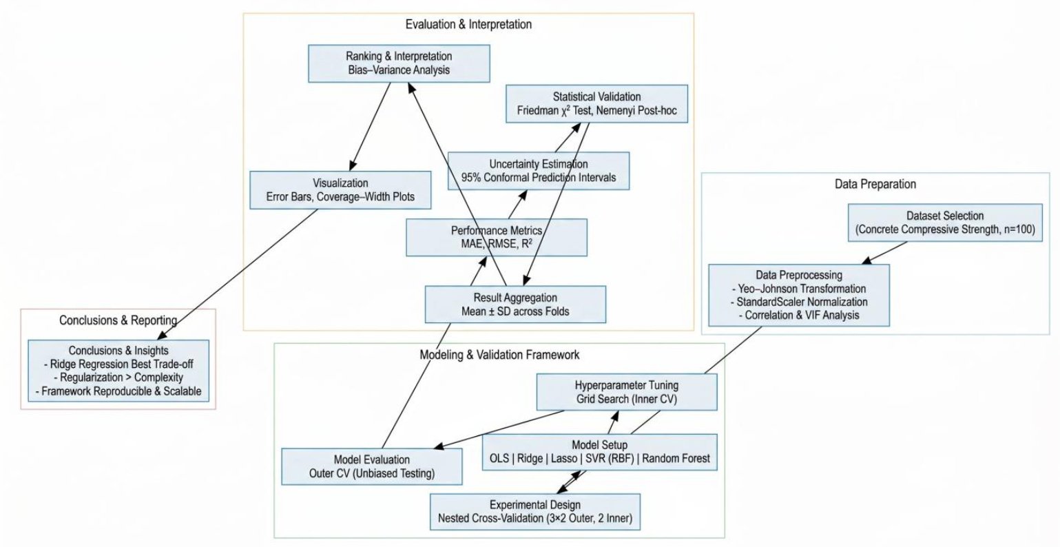
Fig. (1) provides a systematic and repeatable workflow that can be used to test regression models when the sample size is small. It starts with data preprocessing with normalization and correlation analysis to ascertain statistical validity and then takes the nested cross-validation structure, which isolates hyperparameter tuning (inner loop) and unbiased testing (outer loop). There are five benchmarked and modeled models: OLS, Ridge, Lasso, SVR and Random Forest. These evaluation measures (MAE, RMSE, R2) are supplemented by conformal prediction intervals and statistical validation based on the Friedman test. The last phase is the synthesis of findings by aggregating the performances, visualizing performance, and ranking interpretively, which makes Ridge Regression the most trustworthy and understandable model.
3.1. Research Design
The study was quantitative and experimental in nature, to systematically assess the relative predictive accuracy of classical statistical regressors and contemporary machine-learning algorithms when working on small samples. The experimental design construction was carried out in an open-source Python environment with transparency, reproducibility, and accessibility in mind and in Google Colab. The general structure was to create realistic conditions of scarcity of data that are common in engineering and scientific research, where the cost or feasibility of a large-scale data gathering is constrained. Fixed seed initialization (seed = 42) was used to simulate realistic experimental conditions of small sample size. In the preliminary analysis, the experiment was performed with several randomized subsets to assess variability of sampling, and results indicated similarity in the rank of performance across samples. Overview statistics of these pre-test resampling experiments. The 100-sample size was thus maintained as a controlled low-data benchmark and not as a need to reduce data. This sample was also selected on purpose to highlight the issue of overfitting, instability and variance inflation that can occur when models are trained on small datasets.
The experiment was designed on the basis of a comparative study as it was performed on five different algorithms which can be discussed as two modeling paradigms i.e. traditional parametric regressors (OLS, Ridge, Lasso) and non-parametric machine-learning models (Support Vector Regression and Random Forest). Both of the models were evaluated in the light of a nested cross-validation scheme to eliminate information leakage between training and validation phases and provide an objective result on the generalization of models. Conformal prediction was also added to its design to produce uncertainty intervals, measures of the trustworthiness of the predictions of each model. This nonparametric embedded validation and conformal inference is a methodological advance that seeks to address the issues of accuracy and interpretability in small-sample research.
3.2. Sampling Sensitivity Analysis
In order to assess the strength of the experimental results against sampling variability, further experiments of resampling were conducted based on various randomly generated independent subsets of the original data. All the subsets were 100 observations and were generated with various fixed random seeds to guarantee reproducibility but with a varied sample composition. Each resampled dataset was re-trained and tested on the same nested cross-validation procedures. The relative ranking of models, performance trends and the error distributions were mostly similar across sampling iterations. These findings show that the reported results were not specific to one sample realization and are stable with conclusions with small samples.
3.3. Dataset
The dataset adopted in the study was the Concrete Compressive Strength Data Set, publicly available on Kaggle. Previously, machine learning and statistical modeling studies have extensively used it as a benchmark of the performance of regression models, notably in the context of materials engineering. The sample will include 1,030 records concerning the physical and chemical composition of concrete mixtures and their compressive strength in megapascals (MPa). In order to carry out this study, a representative sample of 100 observations was sampled to intentionally induce a small-sample research setting, and not as a necessity because of the data at hand. In order to determine the sampling variability, more sensitivity tests were carried out with several randomly generated independent subsets (all of size n = 100) of the entire dataset with various fixed random seeds. Each model was re-assessed by the same nested cross-validation procedures. These performance rankings, distributions of errors and estimates of uncertainty were found to be consistent across resampled subsets, which suggests that the reported conclusions are not being influenced by one of the sample realizations.
The data has eight independent variables, namely cement, blast-furnace slag, fly ash, water, superplasticizer, coarse aggregate, fine aggregate and age of curing (days). All these variables explain the input items that define the concrete strength. Compressive strength is the dependent variable and a continuous output that is to be predicted. Its strengths range between about 10 Mpa and 80 Mpa, which has a broad dynamic range that can be included in regression analysis. The raw data did not have any values missing, thus making preprocessing and consistency in model input relatively simpler. Nonetheless, exploratory data analysis showed that some of the numerical attributes, including superplasticizer and fly ash contents, have mild skewness, which required normalization to stabilize the variance and enhance model convergence.
This dataset is also physically interpretable, which is one more significant argument why it is selected for the current study. The predictors have a clear engineering definition, allowing one to have a clear understanding of model coefficients and their impact. This dataset serves as a reasonable benchmark on which interpretable statistical models can be compared to opaque machine-learning architectures in a realistic scientific setting.
3.4. Preprocessing
Preprocessing of data was done to improve the reliability of model performance as well as the comparability. Numerical variables were initially converted through the Yeo-Johnson power transformation, which is capable of operating both positive and zero values, hence better than logarithmic scaling when dealing with skewed distributions. In this step, mild asymmetry was fixed and normality was enhanced, which is advantageous to linear and kernel-based algorithms. After transformation, a normalization of the variables was done using z-score scaled with the scikit-learn Standard Scaler, where all the predictors mean of zero and a standard deviation of one. The importance of standardization was especially important when it comes to algorithms like Ridge, Lasso, and SVR that are sensitive to feature scaling. Variance Inflation Factor (VIF) analysis revealed that there was no problem of multicollinearity, with all the values of VIF below 5, thus assuring numerical stability in the linear regression-based models. There were no categorical variables and no code-encoding was required. The outliers were not eliminated intentionally, since they are more consistent with the variability of the real world and allow models to show strength in imperfect data conditions.
3.5. Experimental Framework
The experimental design employed a nested cross-validation (CV) process to give unbiased performance estimates and effective hyperparameter optimization. In a nested CV, there are two loops, one being an inner loop to optimize the model and an outer loop to evaluate without any bias. The outer loop involved a 3-fold CV repeated twice (32), thus 6 outer folds and made sure that every observation was used at a minimum once in the validation. The inner loop used a 2-fold CV on the outer training split to optimize hyperparameters using a grid search.
This architecture eliminates data leakage, which is typical of the traditional single-loop CV, in which the parameters of the model are being optimized with reference to the same data as subsequently used to perform an evaluation. All random processes were also initialized using a fixed random seed to provide reproducibility and erase stochastic variation (42).
Five models were included in the comparison:
- Ordinary Least Squares (OLS) – used as a baseline to evaluate the added value of regularization and nonlinearity.
- Ridge Regression – implemented with an L2 penalty, evaluated over α ∈ {0.1, 1, 10}.
- Lasso Regression – employing L1 regularization, tuned over α ∈ {0.01, 0.1, 1}.
- Support Vector Regression (SVR) – a constrained grid search was intentionally adopted to prevent overfitting under extremely small training folds. Preliminary experiments using broader randomized searches produced comparable rankings but higher variance, therefore a conservative grid was retained to ensure fair comparison across paradigms.
- Random Forest Regression (RF) – an ensemble of decision trees trained with n_estimators ∈ {100, 200} and maximum depth ∈ {3, 5}.
All the pipelines were enclosed with scikit-learn that comprised preprocessing, scaling, and estimator definition. This guaranteed a uniform change in training and test folds, which killed preprocessing bias. The rationale for selecting these five models was to ensure coverage of distinct algorithmic paradigms within regression modeling. OLS is a simple linear model, Ridge and Lasso are regularized linear models that prevent overfitting with L2 and L1 penalty terms, respectively, SVR is a non-linear learner based on a kernel and Random Forest is an ensemble-based, non-parametric model that combines decision trees. These five models, in combination, cover the range of theoretical and methodological variety of classical and modern regression methods, and permit a comparative assessment that is even-handed within the small-sample limitations (Table 1).
Table 1. Model configuration.
| Category | Model | Regularization/Kernel | Key Parameters |
| Statistical | OLS | none | baseline |
| Ridge | L2 | α ∈ {0.1, 1, 10} | |
| Lasso | L1 | α ∈ {0.01, 0.1, 1} | |
| Machine Learning | SVR (RBF) | radial kernel | C ∈ {1, 10}, γ = scale |
| Random Forest | ensemble trees | n = 100–200, depth = 3–5 |
3.6. Evaluation Metrics
3.6.1. Conformal Prediction Framework
This study employed split conformal prediction within each outer fold of the nested cross-validation procedure. For every outer training–validation partition, the regression model was first trained on the outer training subset, and calibration residuals were computed on the corresponding validation fold. The nonconformity score was defined as the absolute residual (Eq. 5):
 (5)
(5)
Prediction intervals were then constructed using the empirical quantile of these residuals, with , yielding 95% marginal coverage. Split conformal prediction is a distribution-free and that it offers a finite-sample, distribution-free coverage guarantee in the case of exchangeability [37].
Further variations like CV+ or jackknife+ conformal prediction were not carried out. Even though this can be used to enhance interval efficiency, it needs repeated model refitting and can inflate the computational variance when the folds are very small. Since nested cross-validation already downsizes effective training per fold, this study used a conservative split conformal design in order to maintain stability and prevent further inflating variances in low-n environments. This option concurs with the best-practices of uncertainty-aware predictive modeling [10, 11].
Each outer fold was predicted and the results were calculated separately and then combined to show mean empirical coverage and average interval width so that unbiased information is provided on the assessment of generalization.
3.7. Implementation
To ensure methodological transparency and reproducibility, implementation was conducted in Python using established open-source libraries. The whole study was done on a Google Colab platform, where it is possible to compute in the clouds and utilize a graphics card. The computational libraries of great importance were scikit-learn (v1.5) to create models and cross-validate them, NumPy (v2.x) to do mathematical operations and Matplotlib (v3.9) to visualize data. The Colab runtime was based on a Tesla T4 and the majority of the models could be executed efficiently using CPU cores since the size of the dataset was relatively small. Hyperparameter optimization and average model time were approximately one minute each. The hyperparameter grids were also selected to be narrow on purpose in a manner that reflected realistic small-sample research practice where large-scale tuning can exaggerate variance and augment selection bias. The preliminary experiment of more general randomized searches had no significant impact on the ranking of performance but rendered the performance more randomized across folds. Therefore, the conservative grids were maintained to make sure that the stability comes first before the most optimality is achieved.
All preprocessing, modeling and evaluation were packaged into structured Python pipelines so as to enable reproducibility and minimize the risk of human error. The open-science best practices are the next step of this modular workflow that allows other researchers to replicate the results, apply workflow framework to other data, or complicate it further to compare the models. The overall methodology, therefore, provides both empirical soundness and computational transparency, which is an efficient foundation of the subsequent analysis of the model performance and comparative findings.
4. RESULTS
4.1. Summary Statistics
The results section reflects the empirical evidence obtained in the framework of the nested cross-validation, along with the conformal prediction on the 100-sample subset of the Concrete Compressive Strength dataset. The data set consisted of an input matrix X (100 8) of eight continuous predictor variables, which included cement, blast-furnace slag, fly ash, water, superplasticizer, coarse aggregate, fine aggregate, and age and a matched output vector y (100 1), which was the target variable compressive strength. After the process of transformation and normalization, the distribution of each feature was approximately symmetric with a normalized skew of about 0.2, showing that the Yeo-Johnson transformation did manage to stabilize the variance and counter the influence of long tails. The average compressive strength in the sample observations was about 36 MPa, which is appropriate compared to the concept of medium-strength concrete that is utilized in the normal civil construction projects.
The preliminary descriptive analysis had validated moderate inter-feature correlations, the highest of which was between cement content and compressive strength (r ≈ 0.78) and between age and strength (r ≈ 0.60) and indicated physically meaningful relationships that are consistent with the previous literature. The features were homogeneous to a standardized scale, which was also comparable across the models and reduced numerical instability in the process of optimization. This preprocessing consistency was important, especially for regularized regression as well as kernel-based algorithms, which are sensitive to feature scaling. The provided overall sample structure, therefore, gave a valid empirical foundation to test the performance of the model complexity and regularization on small sample constraints.
4.2. Model Performance
Table 2 presents a summary of all five models, the Ordinary Least Squares (OLS), Ridge Regression, the Lasso Regression, Support Vector Regression (SVR) with RBF kernel, and the Random Forest (RF) models in terms of nested cross-validation performance. Every metric depicts the average, as well as the standard deviation (SD) of the external folds, which offers a strong indicator of centre tendency and dispersion.
Table 2. Comparative performance.
| Model | MAE ± SD (MPa) | RMSE ± SD (MPa) | R² ± SD | Coverage | Width (MPa) |
| OLS | 6.72 ± 1.29 | 8.69 ± 1.61 | 0.726 ± 0.061 | 0.9449 | 38.79 |
| Ridge | 6.67 ± 1.23 | 8.54 ± 1.48 | 0.735 ± 0.052 | 0.9599 | 40.12 |
| Lasso | 6.81 ± 1.35 | 8.62 ± 1.61 | 0.730 ± 0.060 | 0.9801 | 44.28 |
| SVR (RBF) | 7.88 ± 1.33 | 9.90 ± 1.49 | 0.641 ± 0.067 | 0.9703 | 48.68 |
| Random Forest | 8.69 ± 2.05 | 10.78 ± 2.16 | 0.573 ± 0.121 | 0.9498 | 54.33 |
Even though Ridge Regression had the best average ranking Friedman test revealed that there was no statistically significant difference amongst models (p = 0.406). Accordingly, the results are to be interpreted as an indication of the way of the performance as opposed to the doubtless high quality.
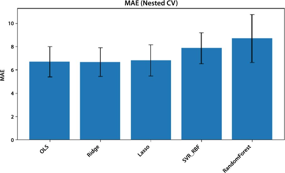
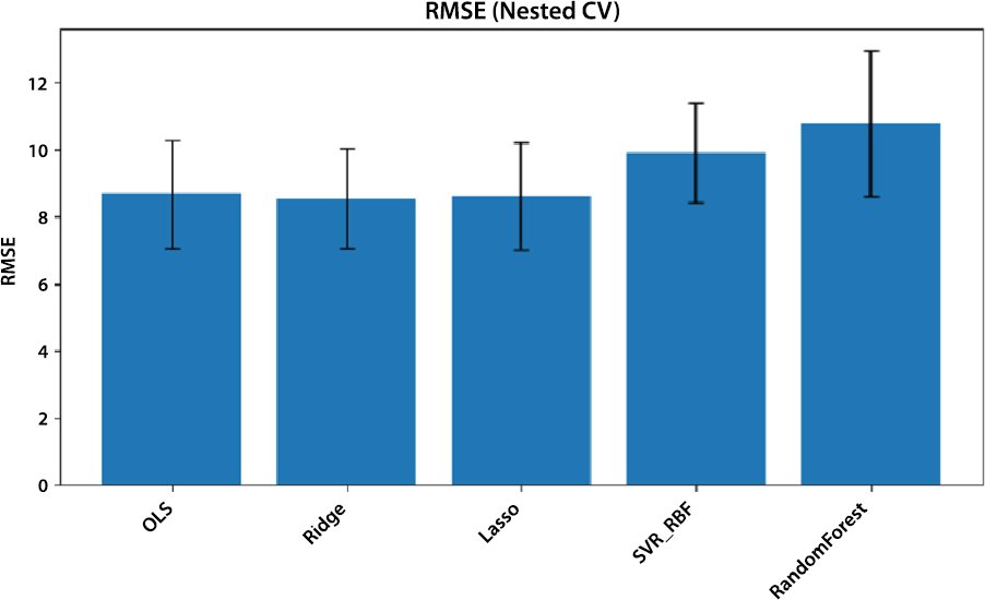
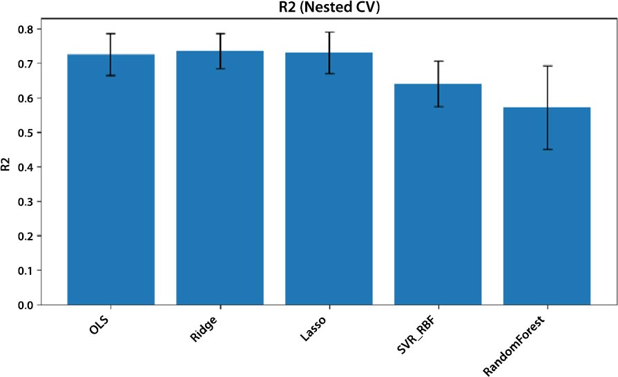
The overall results show that Ridge Regression got the best predictive, and the lowest RMSE (8.54 MPa) with the highest coefficient of determination (R2 = 0.735) followed by Lasso Regression and OLS. These findings confirm the assumption that small-sample conditions favor regularized linear models, compared to machine-learning algorithms of non-linear nature. The OLS, Ridge and Lasso mean absolute errors (MAE) were quite close to 6.7 6.8 MPa and can be proposed that the predictive stability is similar within the folds.
On the other hand, the applied machine-learning models, SVR and Rand Forest, showed much higher errors with the values of RMSE of over 9.9 MPa and over 10.7 MPa, respectively. The fact that the standard deviation of these models has the higher value is also a pointer to the fact that there is some variance in performance of these models when applied to the different segments of the data which is an indication of overfitting. In particular, RMSE variance was the highest using the Random Forest (SD = 2.16), meaning that this algorithm is sensitive to the size of training samples and that it is also sensitive to ensemble diversity that are low when data amounts are also low.
The conformal prediction measures also put into perspective model reliability. Although all models were able to cover the nominal value of 95, which was the required value, the interval width varied considerably. Ridge Regression had a balanced coverage of 0.96 and a moderate average width of 40 Mpa, but Lasso had a slightly higher coverage (0.98) with a slightly wider width of 44 Mpa. Although the coverage of the Random Forest model was 0.95, the intervals were excessively broad with an average of more than 54 MPa- an indication of inflated uncertainty as a result of high variance. These variabilities depict that although ML models can be used to model complex patterns, they cannot learn their uncertainties as accurately in small datasets.
These trends are supported graphically by the comparative bar charts (Figs. 2 and 4). (Fig. 2), MAE plot, indicates that Ridge and OLS give the smallest bars, indicating low errors on average, whereas (Fig. 3), RMSE plot, indicates that there is an apparent distinction between linear and non-linear models, with an error magnitude difference of about 2 MPa. The same hierarchy is reflected in the R2 plot (Fig. 4), with Ridge having the highest percentage of explained variance. Combined, these statistics highlight the regularized linear regressors’ uniform dominance in the predictive and model stability.